
MSAZ-321 · Lesson 9 of 12 · 21 min
Optimizing lakehouse tables
▶ Video coming soon A video version of this lesson is on the way.
On Monday afternoon, November 9, Nikolai and Ines turned from watching the hub to making it faster. DP-700 lists optimizing a lakehouse table first among its performance skills, and MSAZ-320 had already shown the tools: OPTIMIZE, Z-order, V-Order and VACUUM. This session was about deciding when each one helps, measuring the result and keeping tables healthy without anyone having to remember. Ines brought a list of the hub's tables and a question Keiko had asked: why did the same Sales Overview visual take two seconds on Monday and six on Friday?
What makes a Delta table fast or slow
A Delta table is a folder of Parquet files plus a transaction log that lists which files make up the current version. Reading the table means reading the log, choosing the files that might contain the rows a query needs, and reading those files. Three things decide how fast that is. The number of files: every file has a fixed cost to open, so thousands of tiny files are slow even when they hold little data. How well files can be skipped: Delta records the minimum and maximum of columns in each file, by default the first 32 columns, so a query filtering on a column can skip files whose range cannot match, but only if similar values sit together in the same files. And the layout inside each file: V-Order, a Fabric-specific way of sorting and compressing Parquet, makes files faster to read for Power BI, the SQL analytics endpoint and the warehouse, at some cost to write speed.
| Factor | Symptom when poor | Main remedy |
|---|---|---|
| Too many small files | Slow reads despite little data; long query planning | OPTIMIZE, optimize write or auto compaction |
| Poor clustering of filter columns | Queries on one day read every file | Z-order or clustering on the filter columns |
| No V-Order on read-heavy tables | Slower Direct Lake and SQL reads | Enable V-Order for tables read by reports |
| Over-partitioning | Many tiny partitions, each with tiny files | Partition only large tables, on low-cardinality columns |
| Old files never removed | Storage grows; listings slow | VACUUM with a sensible retention |
Measuring a table
Before changing anything, Ines measured. DESCRIBE DETAIL returns a table's number of files, total size, partition columns and properties, and DESCRIBE HISTORY lists each version with its operation, such as WRITE, MERGE or OPTIMIZE, and metrics like files added and removed. Dividing size by number of files gives the average file size, the single most useful health figure. Fabric's guidance is that files of roughly 128 MB to 1 GB read well; files of a few megabytes or less mean the table needs compaction.
detail = spark.sql("DESCRIBE DETAIL lh_curated.sales").collect()[0]
print(detail.numFiles, round(detail.sizeInBytes / 1e9, 2), "GB")

spark.sql("DESCRIBE HISTORY lh_curated.sales").select(
    "version", "timestamp", "operation", "operationMetrics.numAddedFiles", "operationMetrics.numRemovedFiles"
).show(8, truncate=False)| Table | Files | Size | Average file | Verdict |
|---|---|---|---|---|
| lh_curated.sales | 58 | 12.1 GB | About 209 MB | Healthy; 11 small files added since the Nov 2 OPTIMIZE |
| lh_curated.stockline_store_ref | 1 | 0.4 MB | 0.4 MB | Tiny table; one file is fine |
| lh_raw.stockline_sales | 1,183 | 6.8 GB | About 5.7 MB | Needs compaction |
| lh_curated.rejected_rows | 312 | 0.02 GB | About 0.06 MB | Needs compaction; tiny appends every night |
| facilities.freezer_hourly (from tomorrow) | 0 | 0 | – | Plan maintenance before it starts |
The curated sales table was in good shape a week after MSAZ-320's OPTIMIZE: 47 large files plus 11 small ones from the nightly MERGE runs, which was expected. The raw sales table was not: every nightly append and every slice of the history and rerun loads had added files, and the average was under 6 MB. The rejected rows table was worse in proportion but tiny in absolute size, so it mattered little. Keiko's slow Friday visual read the warehouse rather than these tables, and lesson 10 found its cause.
Compaction: OPTIMIZE, optimize write and auto compaction
There are three ways to keep file counts down, and they suit different tables. OPTIMIZE rewrites small files into larger ones after the fact; it is a scheduled job and suits tables that receive many small writes during the week. Optimize write makes each write produce fewer, larger files by reorganizing data before it is written, at the cost of a shuffle during the write; it suits tables written in many partitions or by many tasks. Auto compaction runs a small compaction automatically after a write when it detects enough small files; Fabric's guidance recommends it for new tables that receive frequent small writes, such as streaming ingestion, instead of relying on scheduled OPTIMIZE jobs.
Defaults matter here. New Fabric workspaces use a write-heavy resource profile for Spark, which turns optimize write and V-Order off, favouring fast writes. Other profiles, readHeavyForSpark and readHeavyForPBI, turn on settings that favour reads, and individual settings can be set per session or per table. The hub's curated tables were read far more than they were written, so Nikolai set the readHeavyForPBI profile in the curated environment and left the raw environment write-heavy, matching the V-Order decision from MSAZ-320.
# Raw layer: favour writes, but let small appends compact themselves
spark.conf.set("spark.fabric.resourceProfile", "writeHeavy")
spark.conf.set("spark.databricks.delta.autoCompact.enabled", "true")

# One-off clean-up of the raw sales table
spark.sql("OPTIMIZE lh_raw.stockline_sales")

# Curated environment: favour reads by Power BI and the SQL analytics endpoint
spark.conf.set("spark.fabric.resourceProfile", "readHeavyForPBI")
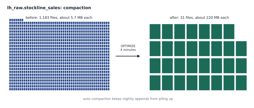
The one-off OPTIMIZE on lh_raw.stockline_sales took four minutes and left 31 files averaging about 220 MB. From then on, auto compaction kept the nightly appends from piling up. For freezer_hourly, which the eventstream's lakehouse destination would write to from the next day in small batches every few minutes, Nikolai chose auto compaction too, plus the weekly maintenance pipeline from MSAZ-320, which already ran OPTIMIZE and VACUUM on the curated tables on Sunday mornings.
Skipping files: Z-order, clustering and statistics
Fewer files help every query; skipping files helps the queries that filter. Delta's per-file statistics let a query on one day skip files that contain no rows for that day, but only if each file holds a narrow range of days. A table loaded in date order is naturally well clustered by date; a table rewritten by MERGE or loaded out of order is not. Z-order, run as part of OPTIMIZE, rearranges rows so that values of one or a few columns are clustered, and newer Delta releases offer liquid clustering, which maintains clustering on chosen columns as data is written and is simpler to change later. Both should be applied to the columns queries filter on most, not to every column.
# Data skipping: how many files must a one-day query read under two layouts?
import random
random.seed(7)
days, files = 1096, 48            # three years of sales days, 48 files after OPTIMIZE

# Unsorted: each file holds rows from days spread across the whole period
unsorted = []
for f in range(files):
    sample = [random.randrange(days) for _ in range(200)]
    unsorted.append((min(sample), max(sample)))   # the file's min and max day

# Sorted by date before writing, as Z-order or clustering on SaleDate would do
per_file = days / files
by_date = [(int(f * per_file), int((f + 1) * per_file) - 1) for f in range(files)]

day = 900                         # the day a store manager asks about
for name, layout in (("unsorted", unsorted), ("sorted by date", by_date)):
    read = sum(1 for lo, hi in layout if lo <= day <= hi)
print(f"{name:15s}: reads {read:2d} of {files} files ({read / files * 100:.0f} in 100)")unsorted : reads 48 of 48 files (100 in 100) sorted by date : reads 1 of 48 files (2 in 100)
What this code does
The program imagines the 48 files of the curated sales table in two layouts. In the unsorted layout each file holds rows from days scattered over three years, so its minimum and maximum day span nearly the whole period; in the sorted layout each file holds a narrow block of consecutive days. For a query about one particular day, it counts how many files have that day within their minimum-to-maximum range and so cannot be skipped. The output shows the unsorted table reading every file and the sorted one reading just one.
The output is the whole argument for clustering in two lines: unsorted, a one-day query reads all 48 files; sorted by date, it reads one. Real tables fall between the two, and MSAZ-320's Z-order on StoreNumber and SaleDate had put the curated table close to the sorted case. Nikolai added a caution. Statistics are collected only for the first 32 columns by default, so a column that queries filter on should not sit at the end of a wide table, and string columns with long values give weaker statistics than dates and numbers.
Partitioning
Partitioning splits a table into folders by a column's value, so queries filtering on that column read only the matching folders. It is powerful for very large tables and harmful for small ones. Each partition holds its own files, so a table partitioned by a column with many values, or a modest table partitioned at all, ends up with many tiny files. A common rule of thumb is to partition only when each partition would hold at least about a gigabyte, on a column with few distinct values that queries nearly always filter on, such as year. The curated sales table, at 12 GB over three years, would have had about 4 GB per year, so partitioning by year was possible but unnecessary given good clustering; partitioning by day, at about 11 MB per day, would have been a mistake.
Checking that it worked
Every optimization should be measured twice, before and after. For the raw table, Ines timed a notebook scan of one month of sales five times before that afternoon's OPTIMIZE and five times after, taking the median of each set: it fell from 48 seconds to 19. For the curated table, Nikolai had kept timings of a query Sales Overview ran often, one store's sales for one week, from before MSAZ-320's OPTIMIZE on November 2; its median had been 3.1 seconds then and was 1.2 now. The figures went into the design table beside each decision, because an optimization nobody can show the effect of is hard to defend when it costs capacity every week.
Worked problem
Should the raw sales table be partitioned by day?
lh_raw.stockline_sales holds 6.8 GB over 1,096 days. If partitioned by day, how large would each partition be? Would that meet a guideline of at least 1 GB per partition, and what about partitioning by year?
Show solution
- Per day: 6.8 GB ÷ 1,096 ≈ 0.0062 GB, about 6.2 MB.
- That is about one-hundred-and-sixtieth of the 1 GB guideline.
- Per year: 6.8 GB ÷ 3 ≈ 2.3 GB, which meets the guideline.
- But queries on raw data rarely filter on year alone, so clustering is the better tool.
Answer: Daily partitions would be about 6 MB each, far too small; yearly partitions would be large enough but bring little benefit, so the table stays unpartitioned and relies on compaction and clustering.
V-Order and the readers
V-Order deserves a decision per table, because its benefit depends on who reads the table. Power BI Direct Lake models, the SQL analytics endpoint and the warehouse read V-Ordered Parquet faster, and the Fabric warehouse writes V-Ordered files by default. Spark reads V-Ordered files normally, without special benefit. Writing with V-Order costs time, so tables written often and read mainly by Spark, such as the raw layer, gain nothing from it. The hub's rule from MSAZ-320 stood: V-Order on for curated tables read by Sales Overview and the SQL endpoint, off for raw tables.
Keeping it automatic
Optimization that depends on someone remembering does not last. The lakehouse offers table maintenance from the explorer, running OPTIMIZE, with V-Order if chosen, and VACUUM on one table; the weekly maintenance pipeline did the same for a list of tables on Sunday mornings; and auto compaction handled the small appends between. Ines added a step to the weekly pipeline that recorded each table's file count and size after maintenance into the load log, so that the monitoring routine from lesson 7 would show a table drifting before anyone felt it.
| Table | Writes | Readers | Maintenance chosen |
|---|---|---|---|
| lh_raw.stockline_sales | Nightly append | Spark notebooks | Auto compaction; weekly OPTIMIZE; no V-Order |
| lh_curated.sales | Nightly MERGE | Sales Overview, SQL endpoint | Weekly OPTIMIZE with Z-order; V-Order; VACUUM 7 days |
| lh_curated.rejected_rows | Tiny nightly appends | Data team | Auto compaction; monthly OPTIMIZE |
| facilities.freezer_hourly | Eventstream every few minutes | Facilities report | Auto compaction; weekly OPTIMIZE; V-Order |
Common mistakes
MistakeRun OPTIMIZE on every table every night.
InsteadMeasure average file size and history; compact the tables that need it, on a schedule that fits their writes.
MistakePartition a table by day because queries filter by day.
InsteadPartition only when partitions would be large; use clustering for selective filters.
MistakeTurn V-Order on everywhere.
InsteadUse V-Order on tables read by Power BI, the SQL endpoint or the warehouse, not on write-heavy raw tables.
MistakePut the most-filtered column at the end of a wide table.
InsteadStatistics cover the first 32 columns by default.
Summary and key terms
- Delta performance depends on file count, how well files can be skipped and the layout inside files.
- DESCRIBE DETAIL and DESCRIBE HISTORY measure a table; average file size is the key health figure.
- OPTIMIZE compacts after the fact, optimize write produces larger files as data is written, auto compaction tidies small writes automatically.
- Resource profiles set write-heavy or read-heavy defaults; new workspaces are write-heavy, with V-Order and optimize write off.
- Z-order or clustering on filter columns lets per-file statistics skip files.
- Partition only large tables on low-cardinality columns; automate maintenance and record its results.
- Small file problem
- Slow reads caused by a table being split into very many small files.
- Optimize write
- A write setting that produces fewer, larger files.
- Auto compaction
- Automatic compaction of small files after writes.
- Data skipping
- Skipping files whose column statistics show they cannot match a filter.
- Liquid clustering
- A Delta feature that keeps data clustered on chosen columns as it is written.
- Resource profile
- A Fabric Spark setting that applies write-heavy or read-heavy defaults.
Practice problems
Work each problem on paper first, then reveal the answer to check.
Which figure did Ines use to judge each table's health?
Show answer
Average file size: total size divided by number of files.
When does Fabric recommend auto compaction?
Show answer
For tables that receive frequent small writes, such as streaming ingestion.
Why did a one-day query on the unsorted model read every file?
Show answer
Every file's date range spanned the whole period, so none could be skipped.
Why not partition the raw sales table by day?
Show answer
Each partition would be about 6 MB, far below the 1 GB guideline.
Which readers benefit from V-Order?
Show answer
Power BI Direct Lake, the SQL analytics endpoint and the warehouse.
Lesson quiz · 5 questions
Score 60% or more to complete this lesson.
Create a free account to save your progress, take quizzes and earn a certificate.