
MSAZ-321 · Lesson 6 of 12 · 21 min
Streaming with Spark structured streaming
▶ Video coming soon A video version of this lesson is on the way.
This morning, Friday, November 13, Ines tried the third streaming engine. The eventstream ingested and routed the freezer readings, and KQL answered questions about them in the eventhouse; Spark structured streaming was the option for teams who want streaming logic in code, written much like the batch notebooks they already had. Facilities had asked for one more table, ten-minute statistics per unit in lh_curated with the minimum, maximum and average and a count of readings, so Ines built it as a structured streaming prototype in FDH Stores [Dev] to see whether the approach suited the hub.
The streaming model
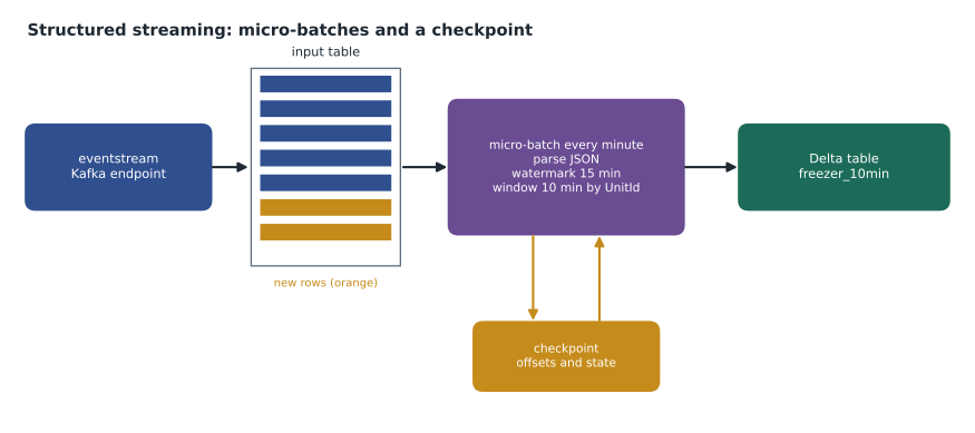
Structured streaming treats a stream as a table that keeps growing. A streaming query is written with the same DataFrame operations as a batch query, select, filter, groupBy and so on, and Spark runs it incrementally: each time new data arrives, it processes only the new rows and updates the result. Under the hood the default engine works in micro-batches, small batch jobs run one after another, each covering the data that arrived since the last. Two things make this reliable. A checkpoint records which data each micro-batch has read and any running state, such as partial aggregates. And a Delta table as the destination, written with a checkpoint, accepts each micro-batch exactly once even if Spark restarts in the middle.
Sources and sinks
In Fabric, a structured streaming query can read from a Delta table, picking up rows as they are appended, which is a common way to move data from a raw table to a curated one continuously. It can read from Azure Event Hubs or from anything that speaks the Kafka protocol, which includes an eventstream's custom endpoint, so a notebook can subscribe to the same events the eventstream carries. Eventstreams also offer a Spark notebook destination, in preview, that wires this up from the eventstream side. The usual destination is a Delta table in a lakehouse.
Kafka sources deliver each event as a row with a binary key and value plus metadata such as the topic, partition, offset and timestamp, so the first step is to cast the value to a string and parse the JSON with a schema. Ines added a custom endpoint destination to the freezer eventstream, read its Kafka connection string from Azure Key Vault in the notebook with notebookutils.credentials.getSecret rather than pasting the secret into a cell, and defined the schema of a reading.
from pyspark.sql import functions as F
from pyspark.sql.types import StructType, StructField, StringType, DoubleType, TimestampType

schema = StructType([
    StructField("UnitId", StringType()),
    StructField("TemperatureC", DoubleType()),
    StructField("ReadingTime", TimestampType()),
])

raw = (spark.readStream.format("kafka")
       .options(**kafka_options)                 # bootstrap servers, topic and SASL settings from the key vault
       .option("startingOffsets", "latest")
       .load())

readings = (raw.select(F.from_json(F.col("value").cast("string"), schema).alias("r"))
               .select("r.*"))
Windows and watermarks
Aggregating a stream by time windows is where structured streaming needs most care, because readings can arrive late. Spark groups by a window function on the event time, for example window(ReadingTime, '10 minutes'), which produces tumbling windows; a third argument makes them sliding. But Spark cannot keep every window open forever waiting for stragglers, or its state would grow without limit. A watermark tells it how late data may be: withWatermark('ReadingTime', '15 minutes') means that once Spark has seen an event time of 8:30, it treats windows that ended before 8:15 as complete, writes their results and drops any later readings for them.
The watermark is a trade-off between completeness and delay. A short watermark finalizes results quickly but drops more late data; a long one keeps more data but holds state longer and finalizes later. The freezer sensors buffer readings during a wireless outage, and facilities had seen outages of up to about twelve minutes, so Ines tested three settings on a model of such outages.
# Event-time windows with a watermark: which late readings still count?
from datetime import datetime as dt, timedelta
base = dt(2026, 11, 13, 8, 0)
buffered = set(range(540, 600, 10)) | set(range(900, 960, 10))
events = [(s, s + 2) for s in range(0, 1800, 10) if s not in buffered]   # normally 2 s late
events += [(s, 1260) for s in range(540, 600, 10)]   # 8:09-8:10, sent at 8:21 after an outage
events += [(s, 1700) for s in range(900, 960, 10)]   # 8:15-8:16, sent at 8:28:20
events.sort(key=lambda e: e[1])                      # process in arrival order

def run(watermark_min):
    latest, counted, dropped = None, {}, 0
    for event_s, arrival_s in events:
        t = base + timedelta(seconds=event_s)
        latest = t if latest is None or t > latest else latest
        watermark = latest - timedelta(minutes=watermark_min)
        window = t.replace(minute=t.minute // 10 * 10, second=0)
        if window + timedelta(minutes=10) <= watermark:
            dropped += 1                              # its window was already finalized
        else:
            counted[window] = counted.get(window, 0) + 1
    return counted, dropped

for w in (2, 10, 15):
    counted, dropped = run(w)
    per_window = ", ".join(f"{k:%H:%M}={v}" for k, v in sorted(counted.items()))
print(f"watermark {w:>2} min: {dropped:>2} readings dropped; {per_window}")watermark 2 min: 12 readings dropped; 08:00=54, 08:10=54, 08:20=60 watermark 10 min: 6 readings dropped; 08:00=54, 08:10=60, 08:20=60 watermark 15 min: 0 readings dropped; 08:00=60, 08:10=60, 08:20=60
What this code does
The program models half an hour of one sensor's readings, one every ten seconds, most arriving two seconds after they were taken, and two minutes of readings held back by wireless outages and sent eleven or twelve minutes late. It processes them in arrival order the way a streaming query does, tracking the latest event time seen, and drops a reading if its ten-minute window has already been closed by the watermark. The output shows, for each watermark length, how many readings were dropped and how many each window ended up with; a complete window has 60.
With a two-minute watermark, both bursts were dropped and two windows were short of their 60 readings. With ten minutes, the burst sent at 8:21 still missed its window, which had closed at 8:20 plus ten minutes of tolerance measured against readings from 8:21, while the second burst was counted. With fifteen minutes, every reading counted. Ines chose fifteen minutes. The cost was that each window's figures would be written about fifteen minutes after it ended, which was fine for a statistics table; the alerting path through Activator did not depend on it.
stats = (readings
         .withWatermark("ReadingTime", "15 minutes")
         .groupBy(F.window("ReadingTime", "10 minutes"), "UnitId")
         .agg(F.min("TemperatureC").alias("MinC"),
              F.max("TemperatureC").alias("MaxC"),
              F.avg("TemperatureC").alias("AvgC"),
              F.count("*").alias("Readings"))
         .select(F.col("window.start").alias("WindowStart"), "UnitId", "MinC", "MaxC", "AvgC", "Readings"))

query = (stats.writeStream
         .format("delta")
         .outputMode("append")
         .option("checkpointLocation", "Files/checkpoints/freezer_10min")
         .trigger(processingTime="1 minute")
         .toTable("facilities.freezer_10min"))
Output modes and triggers
The output mode decides what each micro-batch writes. Append writes only rows that will never change again; with a watermark, that means a window's row is written once, when the window is finalized, which suits a Delta table that other jobs read. Update writes rows that changed in this micro-batch, so a window can be written several times as data arrives, which needs a destination that can update, typically through foreachBatch and a MERGE. Complete rewrites the whole result each time and suits only small aggregates.
The trigger decides when micro-batches run. With no trigger, Spark starts the next micro-batch as soon as the last finishes. A processing-time trigger runs one every fixed interval, such as a minute, which evens out load. An available-now trigger processes everything that has arrived since the last run, in as many micro-batches as needed, and then stops, which turns a streaming query into an efficient incremental batch job that a pipeline or schedule can run every 15 minutes or every hour.
| Setting | Options | Freezer prototype |
|---|---|---|
| Output mode | Append, update, complete | Append, so each window is written once when final |
| Trigger | As soon as possible, processing time, available now | Processing time of 1 minute |
| Watermark | Any duration on the event-time column | 15 minutes, from the longest outages seen |
| Checkpoint | One folder per query, never shared | Files/checkpoints/freezer_10min |
| Sink | Delta table, foreachBatch for MERGE, other sinks | Delta table facilities.freezer_10min |
Checkpoints
Every streaming query needs its own checkpoint location, usually a folder in the lakehouse's Files area. The checkpoint records the source offsets each micro-batch read and the state of running aggregations, so that a restarted query continues exactly where it stopped instead of reprocessing or skipping data. Two rules follow. Never share a checkpoint between queries, because each would overwrite the other's progress. And treat the checkpoint as part of the query: changing the query's logic in incompatible ways, such as the grouping columns, usually needs a new checkpoint and a deliberate decision about where to start reading.
Running a stream for real
A notebook is a good place to develop a streaming query but a poor place to run one permanently, because an interactive session times out and is tied to a person. For a long-running stream, Fabric offers the Spark job definition: an item that runs a main Python or Scala file on a Spark pool, with a retry policy that restarts the job after a failure. Combined with a checkpoint, a restart picks up where the job left off. Streaming jobs also report progress, rows per second processed, batch durations and watermark position, which can be read from the query object and seen in the Spark monitoring pages; lesson 7 covers those.
Cost is the other consideration. A continuously running Spark job holds a session and uses capacity all the time, like an eventstream does. For the freezer statistics, Nikolai did the arithmetic with Ines: a small session running around the clock on the F16 would take a steady share of capacity units for a table that facilities read once a day. The same query with an available-now trigger, run every 15 minutes by a schedule, would produce the same rows with the session running only a minute or two at a time.
Reading a stream's progress
A running query reports on itself after every micro-batch. The query's lastProgress holds the batch number, how many rows arrived, the input and processing rates in rows per second, how long each phase took and the current watermark; recentProgress holds the last few reports. The rule of thumb Nikolai taught was simple: if the processing rate stays below the input rate, the stream is falling behind and the delay will grow until something changes. For the freezer prototype the numbers were tiny, about 1.4 rows a second on average, with short bursts after an outage, and each one-minute micro-batch took about four seconds, so the query was idle most of the time, which was itself the argument for the scheduled available-now version.
p = query.lastProgress
print(p["batchId"], p["numInputRows"], p["inputRowsPerSecond"], p["processedRowsPerSecond"])
print(p["eventTime"].get("watermark"))
Worked problem
Always-on stream or scheduled available-now job?
An always-on session uses an average of 2 CU. An available-now run every 15 minutes takes 90 seconds at 4 CU, including start-up. Compare the CU-seconds per day.
Show solution
- Always on: 2 CU × 86,400 s = 172,800 CU-seconds a day.
- Runs per day: 24 × 4 = 96.
- Scheduled: 96 × 90 s × 4 CU = 34,560 CU-seconds a day.
- \[34{,}560 \div 172{,}800 = 0.2\]
Answer: The scheduled job uses about a fifth of the capacity of the always-on stream, for a table that is read once a day; the figures are illustrative planning numbers.
Which engine for which job
By the end of the morning, Ines had a working prototype and a clearer view of the three engines, which she wrote up for Elena. Eventstreams suit ingestion and light, no-code processing with routing to several destinations. KQL in the eventhouse suits querying and transforming streaming data at scale, with update policies and materialized views. Spark structured streaming suits complex transformation in code, reuse of existing Spark logic, joins with large Delta tables and exactly-once writes to Delta. The hub's decision for the pilot was to keep the eventstream's hourly table, add the ten-minute statistics as a structured streaming query with an available-now trigger scheduled every 15 minutes, and keep the always-on prototype in Dev for the door counters project, where it might be needed later.
| Need | Eventstream | KQL in an eventhouse | Spark structured streaming |
|---|---|---|---|
| No-code ingestion and routing | Best fit | Possible through ingestion | Possible, in code |
| Second-level interactive queries | No | Best fit | No |
| Complex logic, joins with large Delta tables | Limited | Possible | Best fit |
| Exactly-once writes to Delta with custom logic | Lakehouse destination | Through OneLake availability | Best fit |
| Lowest effort for the hub team | Visual editor | KQL to learn | Familiar PySpark |
Common mistakes
MistakeAggregate a stream by time without a watermark.
InsteadAdd a watermark so Spark can finalize windows and limit state.
MistakeShare a checkpoint folder between two queries.
InsteadGive every query its own checkpoint location.
MistakeRun a production stream from an interactive notebook.
InsteadUse a Spark job definition with a retry policy, or an available-now trigger on a schedule.
MistakeGroup by the Kafka timestamp.
InsteadParse the event's own time and window on that.
Summary and key terms
- Structured streaming runs DataFrame queries incrementally in micro-batches over a growing input table.
- Sources include Delta tables, Event Hubs and Kafka-compatible endpoints such as an eventstream's custom endpoint; Delta tables are the usual sink.
- Windows on event time with a watermark balance completeness against delay and bound state.
- Output modes are append, update and complete; triggers are as soon as possible, processing time and available now.
- Each query needs its own checkpoint; restarts continue from it.
- Long-running streams belong in Spark job definitions; available-now triggers make cheap incremental jobs.
- Structured streaming
- Spark's engine for running DataFrame queries incrementally over streams.
- Micro-batch
- A small batch job covering the data that arrived since the last one.
- Watermark
- A limit on how late data may arrive before a window is finalized.
- Checkpoint
- Stored offsets and state that let a streaming query restart where it stopped.
- Output mode
- Whether a streaming query writes final rows, changed rows or the whole result.
- Available-now trigger
- A trigger that processes all available data and then stops.
- Spark job definition
- A Fabric item that runs a Spark program, with a retry policy, outside a notebook.
Practice problems
Work each problem on paper first, then reveal the answer to check.
What does the checkpoint store?
Show answer
The offsets read by each micro-batch and the state of running aggregations.
Why did Ines choose a 15-minute watermark?
Show answer
Outages of up to about twelve minutes buffered readings, and a shorter watermark dropped them.
Which output mode writes each window once, when it is final?
Show answer
Append, with a watermark.
How does an available-now trigger save capacity?
Show answer
It processes what has arrived and stops, so the session runs only briefly on each schedule.
Where should a production stream run?
Show answer
In a Spark job definition with a retry policy.
Lesson quiz · 5 questions
Score 60% or more to complete this lesson.
Create a free account to save your progress, take quizzes and earn a certificate.