
MSAZ-321 · Lesson 10 of 12 · 21 min
Optimizing Spark and warehouse performance
▶ Video coming soon A video version of this lesson is on the way.
After lunch today, Friday, November 13, Nikolai and Ines took on the two performance questions left over from earlier sessions: why nb_clean_sales spent two and a half of its nine minutes starting up, and why Keiko's Sales Overview visual was slow on Fridays. The first was Spark; the second turned out to be the warehouse. Walt Hadley joined for the second half, since the warehouse's T-SQL was familiar ground for a database administrator.
Spark: start-up time
A Spark notebook cannot run until it has a session, and how long that takes depends on the pool and environment. Fabric's starter pools keep warm nodes ready, so a session on a starter pool with no custom libraries usually starts in seconds. A custom pool, or a starter pool with an environment that installs extra libraries, has to provision nodes or install packages first, which takes minutes. nb_clean_sales used an environment with two extra Python libraries, so every run paid about two and a half minutes before the first cell ran.
There were three fixes, and they combined. First, Ines checked whether the libraries were still needed: one, for fuzzy matching of product names, had been replaced by plain PySpark in MSAZ-320, so it came out. Second, high concurrency mode lets notebooks that share the same lakehouse and environment reuse one session; in a pipeline, turning it on for the workspace and giving the notebook activities the same session tag meant nb_setup_dates, nb_clean_sales and nb_clean_products shared one session instead of starting three. Third, the remaining library was small enough to install inline at the start of the notebook during development, while production kept it in the environment.
| Change | Start-up before | Start-up after |
|---|---|---|
| Remove the unused library from the environment | About 150 s | About 95 s |
| Share one session across the three notebooks (high concurrency, session tag) | 3 sessions a night | 1 session a night |
| Total session start-up per night | About 7 minutes | About 1.5 minutes |
Spark: the engine and its settings
Once a session is running, the biggest single setting in Fabric Spark is the native execution engine, which runs Spark SQL and DataFrame operations in a vectorized C++ engine instead of on the Java virtual machine. It is enabled in the environment or per session with spark.native.enabled, and for scan-, filter- and aggregation-heavy work it is often much faster. Not every operation is supported; when one falls back to ordinary Spark, the Spark advisor shows a message in the cell output, which is worth reading because a fallback in the middle of a query can lose most of the benefit.
Adaptive query execution, on by default, adjusts plans while they run: it merges small shuffle partitions after a shuffle, switches a join to a broadcast join when one side turns out to be small, and splits skewed partitions. The default number of shuffle partitions is 200, which suits large data; for a nightly load of a few hundred megabytes, 200 partitions means 200 tiny tasks. Adaptive execution coalesces many of them, but setting spark.sql.shuffle.partitions to a size that fits the data avoids the waste in the first place.
# How many shuffle partitions suit a job? Aim for roughly 128 MB per partition.
target_mb = 128
jobs = {"nightly clean (one day)": 350, "monthly slice backfill": 3_400, "full 3-year rebuild": 41_000}
for name, shuffle_mb in jobs.items():
    default_size = shuffle_mb / 200
    suggested = max(8, round(shuffle_mb / target_mb))
    print(f"{name:26s} shuffle {shuffle_mb:>6,} MB: 200 partitions of {default_size:6.1f} MB;"
          f" suggest about {suggested:>3} partitions")

broadcast_limit_mb = 10            # Spark's default automatic broadcast threshold
for table, mb in {"dim_store": 0.2, "dim_product": 38, "dim_date": 0.3}.items():
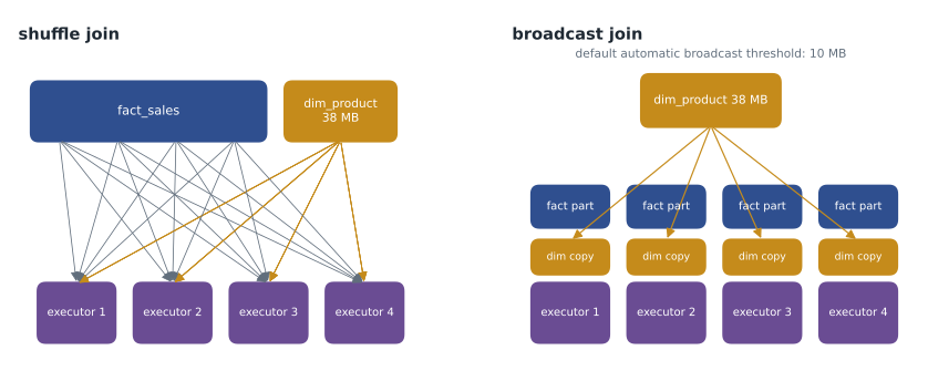
print(f"{table:12s} {mb:>5} MB: {'broadcast automatically' if mb <= broadcast_limit_mb else 'too large for automatic broadcast'}")nightly clean (one day) shuffle 350 MB: 200 partitions of 1.8 MB; suggest about 8 partitions monthly slice backfill shuffle 3,400 MB: 200 partitions of 17.0 MB; suggest about 27 partitions full 3-year rebuild shuffle 41,000 MB: 200 partitions of 205.0 MB; suggest about 320 partitions dim_store 0.2 MB: broadcast automatically dim_product 38 MB: too large for automatic broadcast dim_date 0.3 MB: broadcast automatically
What this code does
The program takes three jobs and the amount of data each one shuffles, and compares Spark's default of 200 shuffle partitions with a count that gives about 128 megabytes per partition, never fewer than eight. It then checks three dimension tables against Spark's default ten-megabyte limit for broadcasting a table to every executor in a join. The output shows that the nightly job's default partitions are under two megabytes each, that the full rebuild needs more than 200, and that the product dimension is too large to broadcast automatically.
The output gave Ines two changes. The nightly notebook set shuffle partitions to 8, leaving adaptive execution to adjust further, and the rebuild notebook, which shuffled about 41 GB, used about 320. And dim_product, at 38 MB, would not broadcast on its own, so the join to it shuffled the whole day's sales; an explicit broadcast hint fixed that, because 38 MB fitted comfortably in each executor's memory. Nikolai warned against copying these numbers to other jobs: the right values come from the Spark UI's stage metrics, not from a rule of thumb.
spark.conf.set("spark.native.enabled", "true")
spark.conf.set("spark.sql.shuffle.partitions", "8")

from pyspark.sql.functions import broadcast
clean = sales_day.join(broadcast(dim_product), "ProductCode", "left")
Spark: skew and memory
Skew is when a few tasks have far more data than the rest, so the stage waits for them. In the Spark UI, a stage whose maximum task time is many times its median is skewed. In the hub, the full rebuild had one: the busiest store, number 4, had about six times as many sales lines as the quietest, and a step grouped by store. Adaptive execution's skew handling splits skewed partitions in joins; for aggregations, adding a second grouping key, such as the day, spreads the work. Memory errors are the other common failure, usually from collecting large results to the driver, caching more than is needed or very wide rows; the spark.task.cpus setting, which defaults to 1, can be raised so that memory-hungry tasks get more of each executor.
| Symptom in the Spark UI | Likely cause | Remedy |
|---|---|---|
| Many tasks of a few milliseconds each | Too many shuffle partitions | Lower shuffle partitions; rely on adaptive execution |
| A few tasks take many times the median | Skewed keys | Skew join handling; add a key to spread aggregation |
| Large shuffle before a join to a small table | No broadcast | Broadcast hint or a higher threshold |
| Executors lost with out-of-memory errors | Collecting or caching too much; memory-hungry tasks | Avoid collect on large data; raise spark.task.cpus |
| Fallback messages in the advisor | Operations the native engine cannot run | Rewrite the operation or accept the fallback |
The warehouse: Keiko's Friday problem
Keiko's slow visual showed each store's sales for the current week against the same week last year. It read a view, wh_sales.dbo.vw_store_week, which Walt had written quickly in MSAZ-320 to test the star schema. Sales Overview was a Direct Lake model, but Direct Lake cannot read a SQL view directly, so visuals on that view fell back to DirectQuery, sending T-SQL to the warehouse each time. On Fridays, when all 23 store managers looked at the week at once, those queries queued.
The warehouse's query insights confirmed it. Every Fabric warehouse has a queryinsights schema with views over its recent history: exec_requests_history lists completed queries with their duration, data scanned and the user; long_running_queries and frequently_run_queries summarize them. Walt filtered exec_requests_history to the last two Fridays: the view's query ran 231 times between 8 and 9 a.m. on November 6, with a median of 5.8 seconds, and each run scanned the whole of fact_sales.
SELECT TOP 10 command, COUNT(*) AS runs,
       AVG(total_elapsed_time_ms) / 1000.0 AS avg_seconds,
       AVG(data_scanned_remote_storage_mb) AS avg_mb_scanned
FROM queryinsights.exec_requests_history
WHERE start_time >= '2026-11-06T14:00' AND start_time < '2026-11-06T15:00'
GROUP BY command
ORDER BY runs DESC;
The view filtered the week with a function applied to the date column, WHERE DATEPART(week, SaleDate) = DATEPART(week, GETDATE()), and a predicate that wraps the column in a function cannot use the column's statistics or the file-level elimination underneath, so every query read every row. Walt rewrote the filter as a range on the integer DateKey, DateKey BETWEEN @week_start AND @week_end, computed once from dim_date, and the scan fell to the fortnight's rows. Then he went further: because the weekly comparison was the same for everyone, he had the nightly load_day procedure maintain a small gold table, gold_store_week, with one row per store per week, which Sales Overview could read in Direct Lake mode with no fallback at all.
| Step | Median time | Data scanned per query |
|---|---|---|
| Original view, function on SaleDate | 5.8 s | All of fact_sales |
| View rewritten with a DateKey range | 1.1 s | About two weeks of rows |
| Gold table read in Direct Lake | Under 0.5 s | One row per store per week |
Warehouse habits
The Fabric warehouse manages much of its own tuning: it maintains statistics automatically, distributes data itself and allocates resources without the resource classes of older SQL products. What remains for the engineer is the design. Statistics can be created or updated manually after a large load if queries run before automatic statistics catch up. Choosing the narrowest data types that fit, such as int keys and varchar of a sensible length rather than varchar(max), shrinks data and speeds joins. Selecting only needed columns matters because storage is columnar. And predicates should compare columns directly, as Walt's fix showed. The first run of a query after a period of quiet can also be slower than later runs, because data must be fetched from OneLake into the warehouse's cache, so performance tests should time several runs, not one.
| Habit | Why |
|---|---|
| Filter on columns, not on functions of columns | Lets statistics and elimination work |
| Narrow data types; avoid varchar(max) for keys | Smaller data, faster joins |
| Select only the columns needed | Columnar storage reads only those columns |
| Pre-aggregate shared, repeated questions into gold tables | One computation instead of hundreds |
| Check queryinsights after a complaint | Shows what ran, how often and how long |
| Time several runs when testing | The first run after a quiet period warms the cache |
Pipelines
Pipelines have their own performance levers, and DP-700 lists optimizing a pipeline separately. Activities with no dependency between them run in parallel, so the shape of the pipeline matters: in pl_nightly_sales, the copy job for small tables already ran alongside copy_sales. ForEach loops run their iterations in parallel up to a batch count, sequentially if Sequential is chosen; the monthly backfill slices in MSAZ-320 used a batch count of 4 to keep capacity use moderate. Copy activities speed up with partitioned reads and parallel copies, as MSAZ-320 showed, and slow down when they wait on a busy source, as lesson 7 found. Small, frequent activities each carry a few seconds of overhead, so combining many tiny steps into one notebook or stored procedure can save more than tuning any of them.
Worked problem
What does sharing a Spark session save?
Three notebooks each started their own session, taking 150, 140 and 130 seconds to start. With high concurrency and a session tag, one session starts in 95 seconds and the other two attach in about 5 seconds each. How much start-up time is saved per night, and over a 30-day month?
Show solution
- Before: 150 + 140 + 130 = 420 seconds, 7 minutes.
- After: 95 + 5 + 5 = 105 seconds, 1.75 minutes.
- Saved per night: 420 − 105 = 315 seconds, 5.25 minutes.
- Per month: 315 × 30 = 9,450 seconds, about 2.6 hours.
Answer: About five and a quarter minutes a night and over two and a half hours a month, with the same results.
Common mistakes
MistakeAccept Spark's default of 200 shuffle partitions for every job.
InsteadSize shuffle partitions to the data, and check the Spark UI.
MistakeJoin a large fact to a 38 MB dimension and wait for a shuffle.
InsteadUse a broadcast hint when the dimension fits in executor memory.
MistakeFilter a warehouse view with a function on the date column.
InsteadCompare the column directly, for example a range on DateKey.
MistakePoint a Direct Lake model at a SQL view and expect Direct Lake speed.
InsteadViews cause DirectQuery fallback; materialize shared results as tables.
Summary and key terms
- Spark start-up depends on the pool and environment; starter pools, fewer libraries and shared high-concurrency sessions shorten it.
- The native execution engine and adaptive query execution speed up most Spark SQL work; the advisor reports fallbacks.
- Size shuffle partitions to the data, broadcast small dimensions and handle skew.
- queryinsights views show a warehouse's recent queries, durations and data scanned.
- Warehouse speed comes from direct predicates, narrow types, column selection and pre-aggregated gold tables.
- Pipelines go faster with parallel branches, sensible ForEach batch counts, partitioned copies and fewer tiny steps.
- Native execution engine
- A vectorized C++ engine that runs Spark operations faster than the JVM.
- Adaptive query execution
- Spark's adjustment of query plans while they run.
- High concurrency mode
- Sharing one Spark session among notebooks with the same lakehouse and environment.
- Broadcast join
- A join that sends a small table to every executor to avoid shuffling the large one.
- Skew
- Uneven data distribution that makes a few tasks far slower than the rest.
- Query insights
- Views in a Fabric warehouse that record recent queries and their performance.
- DirectQuery fallback
- A Direct Lake model sending queries to the SQL engine when it cannot read data directly.
Practice problems
Work each problem on paper first, then reveal the answer to check.
What made nb_clean_sales slow to start?
Show answer
Its environment installed extra libraries, so the session took minutes to start.
How do three notebooks share one session in a pipeline?
Show answer
Turn on high concurrency for the workspace and give the activities the same session tag.
Why was dim_product not broadcast automatically?
Show answer
At 38 MB it was over Spark's default 10 MB threshold.
What did query insights show about the Friday visual?
Show answer
Its query ran 231 times in an hour, took a median 5.8 seconds and scanned all of fact_sales.
Why did the visual's queries go to the warehouse at all?
Show answer
The model read a SQL view, which Direct Lake cannot read, so it fell back to DirectQuery.
Lesson quiz · 5 questions
Score 60% or more to complete this lesson.
Create a free account to save your progress, take quizzes and earn a certificate.