
GEOM-220 · Lesson 9 of 12 · 21 min
Error ellipses
A table of coordinate standard deviations, σE and σN, tells only part of the story of a point's precision. Lesson 2 showed that a point set out by distance and azimuth is much less certain across the line than along it, and that its easting and northing errors are correlated. The standard deviations in easting and northing depend on how the grid happens to be oriented relative to that geometry, and they hide the direction in which the point is weakest. An error ellipse shows the whole picture: the shape, size and orientation of the region in which the true position probably lies. Error ellipses are the standard way of reporting horizontal precision in adjustment reports, and they are what accuracy standards are tested against.
From covariance matrix to ellipse
The precision of a horizontal point is described by the 2 by 2 block of the covariance matrix that belongs to it:
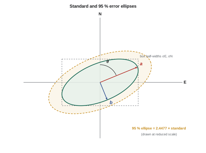
If we ask for the standard deviation of the point's position in some direction at azimuth \(\phi\), the propagation law gives \(\sigma_\phi^2 = \sigma_E^2\sin^2\phi + \sigma_N^2\cos^2\phi + 2\sigma_{EN}\sin\phi\cos\phi\). As \(\phi\) turns through 180°, this has one maximum and one minimum, in perpendicular directions. Those extreme values are the semi-axes of the standard error ellipse, and they are the square roots of the eigenvalues of \(\Sigma\):
The azimuth \(\theta\) of the semi-major axis, measured clockwise from grid north, satisfies
using a two-argument arctangent to put \(2\theta\) in the right quadrant. When the covariance is zero and \(\sigma_E = \sigma_N\), the ellipse becomes a circle and its orientation is undefined. When the covariance is zero but the standard deviations differ, the axes line up with the grid.
Note a subtle point. The semi-major axis is never smaller than either of \(\sigma_E\) and \(\sigma_N\), and the semi-minor axis is never larger. A point can therefore have quite modest coordinate standard deviations and still have a long, thin ellipse leaning at 45°, with a semi-major axis noticeably larger than either. Reporting only σE and σN can understate the worst-direction precision.
Worked problem
Ellipse for a point set out by distance and azimuth
In lesson 2, N1 set out from CR1 had σE² = 36.20 mm², σN² = 10.56 mm² and σEN = −8.22 mm². Find the standard error ellipse.
Show solution
- \[\frac{\sigma_E^2 + \sigma_N^2}{2} = 23.38, \qquad \sqrt{\Big(\frac{36.20 - 10.56}{2}\Big)^2 + (-8.22)^2} = \sqrt{164.4 + 67.6} = 15.23\]
- \[a = \sqrt{23.38 + 15.23} = 6.21\ \text{mm}, \qquad b = \sqrt{23.38 - 15.23} = 2.85\ \text{mm}\]
- \[2\theta = \operatorname{atan2}(2 \times -8.22,\ 10.56 - 36.20) = \operatorname{atan2}(-16.44,\ -25.64) = -147.3^\circ\]
- \[\theta = -73.7^\circ \equiv 106.3^\circ\]
Answer: The semi-major axis is 6.21 mm at an azimuth of 106.3°, exactly perpendicular to the line from CR1, whose azimuth was 16.3°, and its length equals the across-line error d·σα computed in lesson 2. The semi-minor axis is 2.85 mm, the distance standard deviation. The ellipse recovers the physical meaning of the measurement geometry that the coordinate standard deviations had hidden.
Probability and confidence ellipses
The standard ellipse, with semi-axes \(a\) and \(b\), is the two-dimensional counterpart of a one-sigma interval, but it contains much less probability. For a normally distributed position, the probability that the true point lies inside the standard ellipse is only about 39.3 per cent. To enclose a higher probability the ellipse is scaled by a factor \(k\), and for two dimensions
For 95 per cent, \(k = 2.4477\); for 99 per cent, \(k = 3.035\). These come from the chi-square distribution with two degrees of freedom, whose 95 per cent point is 5.991, and \(\sqrt{5.991} = 2.4477\). When the reference variance has been estimated from the adjustment with few degrees of freedom, the factor should strictly come from the F distribution and is larger; with many degrees of freedom it approaches the chi-square value. Most software lets the user choose whether to scale ellipses by the a priori or the a posteriori reference variance, and the report should say which was used.
| Probability | One dimension (k) | Two dimensions (k) |
|---|---|---|
| 39.3 % | 0.51 | 1.000 |
| 50 % | 0.674 | 1.177 |
| 68.3 % | 1.000 | 1.515 |
| 95 % | 1.960 | 2.448 |
| 99 % | 2.576 | 3.035 |
A common mistake is to scale a standard ellipse by 1.96 and call it a 95 per cent ellipse. The result encloses only about 85 per cent. Since accuracy standards are stated at 95 per cent, using the wrong factor understates the true uncertainty by about 20 per cent and could make a survey appear compliant when it is not.
Circular measures
Some specifications use a single radius rather than an ellipse. Circular error probable (CEP) is the radius of a circle containing 50 per cent of positions, roughly \(0.59(a + b)\) for moderately elongated ellipses. Distance root mean square, \(\text{DRMS} = \sqrt{\sigma_E^2 + \sigma_N^2}\), is used in navigation; twice DRMS contains between about 95 and 98 per cent depending on the ellipse shape. North American positioning standards define horizontal accuracy by a 95 per cent confidence measure; the FGDC standard uses the radius of a 95 per cent circle, which for a circular error distribution is \(2.4477\sigma\) and for an elongated ellipse is computed by approximation formulas given in the standard. These are convenient single numbers, but the ellipse remains the more informative description.
Relative error ellipses
For most engineering work, what matters is not how well a point is known relative to the fixed control, but how well two points are known relative to each other. A bridge contractor setting out the two abutments cares about the distance and direction between them, not about their position relative to a national datum many kilometres away. The relative error ellipse describes the precision of the coordinate differences between two points. Its covariance matrix follows from the propagation law applied to \(\Delta E = E_2 - E_1\) and \(\Delta N = N_2 - N_1\):
where \(\Sigma_{12}\) is the 4 by 4 covariance matrix of \((E_1, N_1, E_2, N_2)\). Multiplying out, the variance of \(\Delta E\) is \(\sigma_{E_1}^2 + \sigma_{E_2}^2 - 2\sigma_{E_1E_2}\), and similarly for \(\Delta N\).
The covariance terms between the two points are essential. Neighbouring points in a network are usually positively correlated, because they were fixed by many of the same observations, and the relative ellipse is then smaller than either absolute ellipse would suggest. Ignoring the correlation and simply adding the two points' variances gives a pessimistic answer, sometimes by a large margin. The program below works out the full off-diagonal term with the Jacobian rather than writing it by hand.
Relative ellipses are drawn at the midpoint of the line joining the two points. A good network has relative ellipses that are small and roughly circular between every pair of points that must be set out from one another. A relative ellipse elongated along a line points to a weak distance connection; one elongated across the line points to weak angular connection.
def T(A): return [list(r) for r in zip(*A)]
def mul(A, B): return [[sum(a * b for a, b in zip(r, c)) for c in zip(*B)] for r in A]
def inv(A):
    n = len(A); M = [list(map(float, r)) + [1.0 if i == j else 0.0 for j in range(n)] for i, r in enumerate(A)]
    for c in range(n):
        p = max(range(c, n), key=lambda r: abs(M[r][c])); M[c], M[p] = M[p], M[c]
        d = M[c][c]; M[c] = [x / d for x in M[c]]
        for r in range(n):
            if r != c:
                f = M[r][c]; M[r] = [x - f * y for x, y in zip(M[r], M[c])]
    return [r[n:] for r in M]
def diag(v): return [[v[i] if i == j else 0.0 for j in range(len(v))] for i in range(len(v))]
def col(v): return [[x] for x in v]
# Absolute and relative error ellipses from the bridge network covariance matrix
import math

# Covariance matrix of (E_N1, N_N1, E_N2, N_N2) from lesson 8, in mm^2
C = [[6.5471, 0.9370, 4.3057, -0.8069],
     [0.9370, 6.4101, 1.3241, -0.0006],
     [4.3057, 1.3241, 7.3937, -1.6283],
     [-0.8069, -0.0006, -1.6283, 6.3608]]

def ellipse(sEE, sNN, sEN):
    mid = (sEE + sNN) / 2
    rad = math.sqrt(((sEE - sNN) / 2) ** 2 + sEN ** 2)
    a, b = math.sqrt(mid + rad), math.sqrt(mid - rad)
    az = math.degrees(0.5 * math.atan2(2 * sEN, sNN - sEE)) % 180   # azimuth of major axis
    return a, b, az

K95_2D = math.sqrt(-2 * math.log(1 - 0.95))      # 2.4477 for a 95 per cent ellipse
print(f"95 per cent scale factor for two dimensions = {K95_2D:.4f} (1.96 in one dimension)")

for name, i in (('N1', 0), ('N2', 2)):
    a, b, az = ellipse(C[i][i], C[i + 1][i + 1], C[i][i + 1])
    print(f"{name}: standard ellipse a = {a:.2f} mm, b = {b:.2f} mm, major axis azimuth {az:.1f} deg;"
          f" 95 per cent a = {K95_2D * a:.1f} mm, b = {K95_2D * b:.1f} mm")

# Relative ellipse N1 -> N2: covariance of (E2 - E1, N2 - N1)
J = [[-1, 0, 1, 0], [0, -1, 0, 1]]
R = [[sum(J[p][i] * C[i][j] * J[q][j] for i in range(4) for j in range(4)) for q in range(2)] for p in range(2)]
a, b, az = ellipse(R[0][0], R[1][1], R[0][1])
d = math.hypot(5530.0001 - 5119.9999, 5459.9993 - 5409.9994)
print(f"relative N1-N2: a = {a:.2f} mm, b = {b:.2f} mm, azimuth {az:.1f} deg, 95 per cent a = {K95_2D * a:.1f} mm")

# Compare with a relative positional precision of 20 mm + 50 ppm at 95 per cent
allow = 20 + 50e-6 * d * 1000
print(f"line length {d:.1f} m: allowable {allow:.1f} mm, achieved {K95_2D * a:.1f} mm ->",
      "meets" if K95_2D * a <= allow else "fails")

# Probability inside a circle of radius k*sigma for a circular 2D error
for k in (1.0, 1.1774, 2.0, 2.4477, 3.0):
print(f"radius {k:.4f} sigma contains {100 * (1 - math.exp(-k * k / 2)):.1f} per cent")95 per cent scale factor for two dimensions = 2.4477 (1.96 in one dimension) N1: standard ellipse a = 2.72 mm, b = 2.35 mm, major axis azimuth 47.1 deg; 95 per cent a = 6.7 mm, b = 5.8 mm N2: standard ellipse a = 2.93 mm, b = 2.27 mm, major axis azimuth 126.2 deg; 95 per cent a = 7.2 mm, b = 5.6 mm relative N1-N2: a = 3.60 mm, b = 2.27 mm, azimuth 171.0 deg, 95 per cent a = 8.8 mm line length 413.0 m: allowable 40.7 mm, achieved 8.8 mm -> meets radius 1.0000 sigma contains 39.3 per cent radius 1.1774 sigma contains 50.0 per cent radius 2.0000 sigma contains 86.5 per cent radius 2.4477 sigma contains 95.0 per cent radius 3.0000 sigma contains 98.9 per cent
Both new points in the bridge network have nearly circular ellipses, with semi-axes of about 2.3 to 2.9 mm, which reflects the good mix of distances and angles from two well-placed pillars. The relative ellipse between N1 and N2 has a semi-major axis of 3.6 mm, at an azimuth of 171°, almost perpendicular to the line between them, whose azimuth is 83°. The weaker relative direction is therefore across the line, which is controlled by the angles, while the measured distance N1–N2 holds the along-line component tightly. At 95 per cent the semi-major axis is 8.8 mm. The relative variance in easting, 5.3 mm², is smaller than either point's own easting variance because the two points are positively correlated in easting.
Comparing with accuracy standards
In Canada, the Geodetic Survey of Canada's Accuracy Standards for Positioning define network accuracy, relative to the national reference frame, and local accuracy, relative to neighbouring points, both at 95 per cent confidence. Provincial standards, such as the Alberta Land Surveyors' Association Manual of Standard Practice, build on the same 95 per cent idea. The bridge project specification required local accuracy between control points of 10 mm at 95 per cent; the relative ellipse between N1 and N2, at 8.8 mm, meets it.
The program also checks the N1–N2 line against a 2 cm + 50 ppm standard of the kind used for boundary surveys. With an allowance of 40.7 mm on a 413 m line, the 8.8 mm achieved is comfortable. In many engineering applications the project specification is far tighter than boundary standards, and it is the project specification that must govern.
Two cautions apply to every such comparison. First, the ellipses come from the a priori or a posteriori stochastic model, so they are only as realistic as the weights. An adjustment with optimistic standard deviations will produce small ellipses and a false impression of compliance, which is why the global test of lesson 10 should pass before the ellipses are quoted. Second, ellipses describe random error only. A systematic error, such as an incorrect combined scale factor or a disturbed control point, does not enlarge them at all.
Common mistakes
MistakeScaling a standard ellipse by 1.96 for 95 per cent.
InsteadUse 2.4477 for a two-dimensional 95 per cent ellipse.
MistakeReporting only σE and σN.
InsteadReport the semi-axes and orientation of the ellipse, which show the worst direction.
MistakeComputing relative precision without covariances between points.
InsteadInclude the covariance terms; neighbouring points are usually correlated.
MistakeQuoting ellipses from an adjustment that failed its global test.
InsteadFix the stochastic model or the data first; ellipses depend on the weights.
MistakeAssuming small ellipses mean an accurate survey.
InsteadEllipses show precision only; systematic errors and bad control are not included.
Summary and key terms
- The standard error ellipse has semi-axes equal to the square roots of the eigenvalues of the point's 2 × 2 covariance matrix.
- The major axis azimuth satisfies tan 2θ = 2σEN / (σN² − σE²).
- The standard ellipse contains only 39.3 per cent probability.
- A 95 per cent ellipse is the standard ellipse scaled by 2.4477.
- Relative ellipses describe the precision between two points and need their covariances.
- North American accuracy standards compare 95 per cent measures with allowable values.
- Ellipses reflect random errors and the stochastic model, not systematic errors.
- Standard error ellipse
- The ellipse whose semi-axes are the maximum and minimum standard deviations of a position.
- Confidence ellipse
- A standard ellipse scaled to contain a stated probability.
- Relative error ellipse
- An ellipse describing the precision of the coordinate differences between two points.
- Eigenvalue
- A value λ for which a matrix multiplied by a vector equals λ times that vector; here the squared semi-axes.
- Circular error probable
- The radius of a circle containing 50 per cent of positions.
- Local accuracy
- The accuracy of a point relative to neighbouring points, at 95 per cent confidence.
Practice problems
Work each problem on paper first, then reveal the answer to check.
A point has σE = σN = 4 mm and σEN = 0. Describe its standard ellipse.
Show answer
A circle of radius 4 mm.
A point has σE² = 9, σN² = 4 and σEN = 0 (mm²). Give a, b and θ.
Show answer
a = 3 mm, b = 2 mm, θ = 90° (major axis east-west).
What is the 95 per cent semi-major axis for a = 3.2 mm?
Show answer
2.4477 × 3.2 = 7.8 mm.
What probability does a standard ellipse scaled by 2 contain?
Show answer
1 − e⁻² = 86.5 per cent.
What is the allowable relative precision on a 250 m line at 2 cm + 50 ppm?
Show answer
20 + 12.5 = 32.5 mm.
Lesson quiz · 5 questions
Score 60% or more to complete this lesson.
Create a free account to save your progress, take quizzes and earn a certificate.