
GEOM-220 · Lesson 3 of 12 · 21 min
Weights and precision
Lesson 1 averaged ten measurements that were all made the same way, so each deserved the same say in the result. Real survey data is rarely so uniform. A benchmark height may be carried in by three level routes of different lengths; an angle may be measured with two sets by one crew and six by another; a network may combine total station distances of 80 m and 1,200 m with GNSS baselines of 15 km. A long level line is less precise than a short one, and an angle from six sets is better than one from two. Weights are how least squares gives each observation the influence its precision deserves. This lesson defines weights, shows how they are chosen for the common kinds of survey measurement, and introduces the weighted mean, which is the simplest least squares adjustment of all.
What a weight is
The weight of an observation is inversely proportional to its variance:
Here \(\sigma_0^2\) is a constant called the reference variance, or variance of unit weight. It can be chosen freely, because only the ratios between weights affect the adjusted values. An observation whose variance equals \(\sigma_0^2\) has a weight of exactly one. Choosing \(\sigma_0\) to be a round number for a typical observation, such as 1 mm for a one-kilometre level line, keeps the weights easy to read.
Two observations with variances in the ratio 1 to 4 (standard deviations of 1 mm and 2 mm) have weights in the ratio 4 to 1. The more precise observation has four times the influence, not twice, because weights follow variances and not standard deviations. This catches many students out. Halving the standard deviation of an observation quadruples its weight.
Weights have units. If \(\sigma_0\) is in millimetres and an angle's \(\sigma\) is in seconds, the weight carries units of mm² per square second. That is no problem inside a single adjustment, as long as the residuals are expressed in consistent units, but it is one reason that mixed networks are best handled with the covariance matrix described later in this lesson.
Choosing weights for survey measurements
Weights come from the expected precision of each observation, which in turn comes from the instrument specification, the field procedure and experience. A few standard cases cover most survey work.
| Observation | Variance model | Usual weight |
|---|---|---|
| Levelled height difference | σ² = k²K, with K the length in km | w = 1/K (σ0 = k per √km) |
| Line levelled with n set-ups | σ² = n σ²(set-up) | w = 1/n |
| Mean of n sets of an angle or direction | σ² = σ²(set)/n | w = n |
| EDM distance | σ² = (a + b·d)² or a² + (b·d)², plus centring | w = σ0²/σ²(d) |
| GNSS baseline component | From the processing covariance matrix, often scaled | Full 3×3 weight block |
| Mean of n equal measurements | σ² = σ²/n | w = n |
Levelling is the textbook case. Lesson 2 showed that the standard deviation of a levelled height difference grows with the square root of the number of set-ups, and therefore roughly with the square root of the distance. The variance grows with the distance itself, so the weight is the reciprocal of the length in kilometres. A route of 0.5 km has a weight of 2; a route of 4 km has a weight of 0.25. In rough country, where sights are short and set-ups are many, weights by the number of set-ups are more realistic than weights by length.
EDM distances have a constant part, from the instrument's internal electronics and from centring the instrument and reflector, and a part proportional to the distance, from the frequency and atmospheric corrections. The manufacturer's specification, such as 2 mm + 2 ppm, is a starting point. Many offices combine the parts in quadrature and add centring errors of about 1 mm at each end, giving \(\sigma_d^2 = a^2 + (b\,d)^2 + \sigma_{c,i}^2 + \sigma_{c,t}^2\). For short lines the constant terms dominate and every distance has nearly the same weight. For lines of several kilometres the ppm term takes over.
Angles and directions need the same care. A direction measured with a 3″ instrument has a pointing and reading standard deviation of about 3″ per set, but on short sights the effect of centring errors on the angle can be much larger. A 1 mm centring error at a 50 m target causes an angular error of about 4″, more than the instrument itself. Adjustment software that models only the instrument specification will give short sights too much weight.
The weighted mean
When one quantity has been measured several times with different precisions, the best estimate is the weighted mean:
It reduces to the ordinary mean when all weights are equal. Its standard deviation is
which follows directly from the propagation law applied to the formula above. The weighted mean is itself a least squares estimate: it is the value that minimizes the weighted sum of squared residuals \(\sum w_i v_i^2\). Lesson 4 proves that and generalizes it.
Worked problem
Weighted mean of three level routes
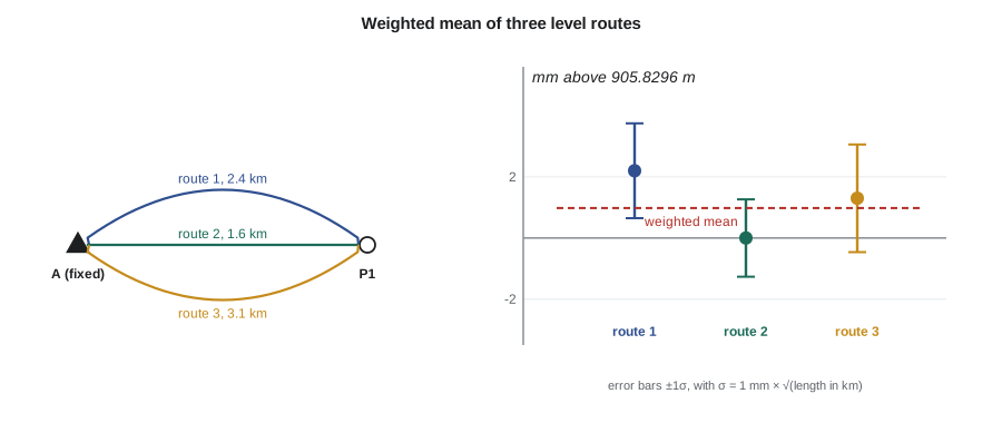
Leah carries the elevation of a new benchmark, P1, at the Coulee Ridge subdivision from benchmark A by three independent routes. Route 1 is 2.4 km long and gives 905.8318 m; route 2 is 1.6 km and gives 905.8296 m; route 3 is 3.1 km and gives 905.8309 m. The levelling standard is 1 mm per √km. Find the weighted mean and its standard deviation.
Show solution
- \[w_1 = \frac{1}{2.4} = 0.4167, \quad w_2 = \frac{1}{1.6} = 0.6250, \quad w_3 = \frac{1}{3.1} = 0.3226, \quad \sum w = 1.3642\]
- \[\bar{H} = 905.8296 + \frac{0.4167(2.2) + 0.6250(0) + 0.3226(1.3)}{1.3642}\ \text{mm} = 905.8296 + 0.98\ \text{mm} = 905.8306\ \text{m}\]
- \[v_1 = -1.2\ \text{mm}, \quad v_2 = +1.0\ \text{mm}, \quad v_3 = -0.3\ \text{mm}\]
- \[\sigma_{\bar{H}} = \frac{1.0}{\sqrt{1.3642}} = 0.86\ \text{mm}\]
Answer: The weighted mean is 905.8306 m with a standard deviation of about 0.9 mm. It is closer to route 2's value because route 2 is the shortest and most precise. The unweighted mean would have been 905.8308 m, only 0.2 mm different here, but with routes of very different lengths the difference can be several millimetres. In lesson 7 this same benchmark is adjusted as part of a whole network.
The working in the second step uses a trick worth copying. Subtracting a convenient round value (here the smallest observation) before averaging, and adding it back afterwards, keeps the numbers small and avoids rounding problems on a calculator. Software does not need this, but people checking software output by hand do.
A priori and a posteriori reference variance
The reference variance \(\sigma_0^2\) chosen before the adjustment is called the a priori value. After the adjustment, the residuals give an independent estimate called the a posteriori reference variance:
where \(r\) is the number of degrees of freedom, or redundancy: the number of observations minus the number of unknowns. For a weighted mean of \(n\) observations, \(r = n - 1\). If the weights were realistic, \(\hat{\sigma}_0\) should be close to the a priori \(\sigma_0\). A value much larger suggests that the observations were less precise than assumed, or that one contains a blunder; a value much smaller suggests the a priori standard deviations were too pessimistic. Lesson 10 turns this comparison into a formal chi-square test. For the three routes, \(\sum w v^2 = 0.4167(1.22)^2 + 0.6250(0.98)^2 + 0.3226(0.32)^2 = 1.25\) mm², and with two degrees of freedom \(\hat{\sigma}_0 = \sqrt{1.25/2} = 0.79\) mm per √km, comfortably consistent with the assumed 1 mm.
The a posteriori value is often used to scale the precision of the results. The standard deviation of the weighted mean can be reported either as \(\sigma_0/\sqrt{\sum w}\), trusting the a priori model, or as \(\hat{\sigma}_0/\sqrt{\sum w}\), trusting the data. With only two degrees of freedom the a posteriori estimate is itself very uncertain, so most practitioners use the a priori value unless the global test fails. With large networks, where hundreds of degrees of freedom make \(\hat{\sigma}_0\) reliable, scaling by it is common.
# Weighted mean of a benchmark height from three level routes
import math

routes = [  # (elevation in m, route length in km)
    (905.8318, 2.4),
    (905.8296, 1.6),
    (905.8309, 3.1),
]
sigma0 = 1.0                               # mm per square-root km, a priori
w = [1 / k for _, k in routes]
H = [h for h, _ in routes]
Hw = sum(wi * hi for wi, hi in zip(w, H)) / sum(w)
v = [(Hw - hi) * 1000 for hi in H]         # residuals in mm
r = len(H) - 1                             # degrees of freedom
s0_post = math.sqrt(sum(wi * vi ** 2 for wi, vi in zip(w, v)) / r)

print(f"weights: {', '.join(f'{x:.4f}' for x in w)}  (sum {sum(w):.4f})")
print(f"weighted mean = {Hw:.4f} m, ordinary mean = {sum(H) / len(H):.4f} m")
print("residuals (mm):", ", ".join(f"{x:+.2f}" for x in v))
print(f"sum of w*v = {sum(wi * vi for wi, vi in zip(w, v)):.6f} (zero for a weighted mean)")
print(f"a priori sigma of mean  = {sigma0 / math.sqrt(sum(w)):.2f} mm")
print(f"a posteriori sigma0 = {s0_post:.2f} mm/sqrt(km) with {r} degrees of freedom")
print(f"a posteriori sigma of mean = {s0_post / math.sqrt(sum(w)):.2f} mm")

# Angle measured with different numbers of sets (weight = number of sets)
sets = [(52.0, 2), (53.9, 4), (53.2, 6)]   # seconds part of 32 deg 43 min, sets
wa = sum(n * s for s, n in sets) / sum(n for _, n in sets)
print(f"weighted angle = 32 deg 43 min {wa:.2f} sec, sigma = {3 / math.sqrt(12):.2f} sec for 12 sets of 3 sec")weights: 0.4167, 0.6250, 0.3226 (sum 1.3642) weighted mean = 905.8306 m, ordinary mean = 905.8308 m residuals (mm): -1.22, +0.98, -0.32 sum of w*v = 0.000000 (zero for a weighted mean) a priori sigma of mean = 0.86 mm a posteriori sigma0 = 0.79 mm/sqrt(km) with 2 degrees of freedom a posteriori sigma of mean = 0.68 mm weighted angle = 32 deg 43 min 53.23 sec, sigma = 0.87 sec for 12 sets of 3 sec
Two checks in the output are worth making a habit. The weighted sum of the residuals is zero, which is the weighted counterpart of the ordinary residuals summing to zero, and is a quick test that the arithmetic is right. And the a posteriori reference standard deviation, 0.79 mm per √km, is close to the 1 mm assumed, so the levelling behaved as expected and the weights were sensible.
Covariance, cofactor and weight matrices
When observations are correlated, as GNSS baseline components are, or when there are many of them, the weights are collected into a weight matrix. Starting from the covariance matrix of the observations \(\Sigma_{\ell\ell}\), the cofactor matrix is the covariance matrix divided by the reference variance, and the weight matrix is its inverse:
For uncorrelated observations \(\Sigma_{\ell\ell}\) is diagonal and \(\mathbf{P}\) simply has the individual weights on its diagonal. For three independent level routes,
For a GNSS baseline, the processing software supplies a full 3 by 3 covariance matrix for the three components, with substantial correlations between them, and its inverse is a full 3 by 3 block in \(\mathbf{P}\). Dropping the off-diagonal terms would discard real information about the geometry of the solution. Note also that GNSS processing software is known to report formal precisions that are too optimistic, often by a factor of several, because it does not model all error sources; a scaling factor determined from experience or from the network adjustment's own reference variance is normally applied.
Weights in combined networks
Networks that mix observation types depend on weights more than anything else. If the distances in a trilateration network are given realistic standard deviations but the angles are given standard deviations that are too small, the adjustment will bend the distances to fit the angles, and the residuals of the distances will look suspicious even though the fault lies with the angle weights. A practical method used in many offices is to adjust each observation type alone first, check that its reference variance is near one, and only then combine them. Variance component estimation is a formal version of this idea, which estimates a separate scale factor for each group of observations; it is beyond the scope of this course but is built into most professional adjustment packages.
Weights also encode judgement. A distance measured in shimmering heat at midday, or an angle to a target the crew noted as poorly lit, may deserve a reduced weight. That decision should be recorded in the field notes and the adjustment report, so that anyone reviewing the work can see why the observation was treated differently. Changing weights after the fact simply to make the statistics look better is not acceptable practice.
Common mistakes
MistakeMaking weights proportional to standard deviations.
InsteadMake them inversely proportional to variances: halving σ quadruples the weight.
MistakeWeighting long and short level lines equally.
InsteadWeight level lines by 1/length in km, or by 1/number of set-ups in rough terrain.
MistakeUsing only the instrument's angle specification on short sights.
InsteadInclude centring errors, which dominate on short lines.
MistakeThrowing away GNSS baseline correlations.
InsteadUse the full 3 × 3 covariance block, scaled if necessary.
MistakeChanging weights to make statistics pass.
InsteadChange weights only with a documented physical reason.
Summary and key terms
- Weights are inversely proportional to variances: w = σ0²/σ².
- Only the ratios of weights affect adjusted values; σ0 sets the scale.
- Levelled lines are weighted by 1/K; angle means by the number of sets.
- The weighted mean is Σwx/Σw with standard deviation σ0/√Σw.
- The a posteriori reference variance Σwv²/r checks whether the weights were realistic.
- The weight matrix is the inverse of the cofactor matrix, P = σ0²Σ⁻¹.
- Correlated observations such as GNSS baselines need full weight blocks.
- Weight
- A number inversely proportional to an observation's variance that sets its influence in an adjustment.
- Reference variance
- The variance of an observation of unit weight, written σ0².
- Weighted mean
- The mean in which each observation is multiplied by its weight.
- Redundancy
- The number of observations minus the number of unknowns; the degrees of freedom.
- A posteriori reference variance
- The estimate of σ0² computed from the residuals after an adjustment.
- Cofactor matrix
- The covariance matrix divided by the reference variance.
- Weight matrix
- The inverse of the cofactor matrix of the observations.
Practice problems
Work each problem on paper first, then reveal the answer to check.
Two distances have σ = 3 mm and σ = 6 mm. What is the ratio of their weights?
Show answer
4 to 1.
Give the weights of level routes of 0.8 km and 2.0 km.
Show answer
1.25 and 0.5.
An angle is measured as 45°10′12″ with 3 sets and 45°10′16″ with 1 set. What is the weighted mean?
Show answer
\((3 \times 12 + 1 \times 16)/4 = 13''\), so 45°10′13″.
Four observations with weights summing to 6.25 have σ0 = 2 mm. What is σ of the weighted mean?
Show answer
\(2/\sqrt{6.25} = 0.8\) mm.
An adjustment with 12 degrees of freedom gives Σwv² = 30. What is the a posteriori σ0?
Show answer
\(\sqrt{30/12} = 1.58\).
Lesson quiz · 5 questions
Score 60% or more to complete this lesson.
Create a free account to save your progress, take quizzes and earn a certificate.