
GEOM-220 · Lesson 5 of 12 · 22 min
Observation equations
The observation equation method, also called the parametric method or adjustment by indirect observations, is the workhorse of survey adjustment. Almost every commercial package uses it, because it handles any mix of observation types in a uniform way. The idea is simple: write one equation for each observation, expressing what that observation should be as a function of the unknown coordinates or heights. Lesson 4 did this for linear problems. Here we extend it to the non-linear equations that describe distances and directions, by linearizing them about approximate values and iterating. By the end of the lesson Leah will have computed the position of the bridge control point N1 from four distances, with a full statement of its precision.
The general form
For each observation \(\ell_i\) there is a function \(F_i\) of the unknowns \(\mathbf{x}\) that gives its true value. The adjusted observation equals that function evaluated at the adjusted unknowns:
With \(n\) observations and \(u\) unknowns there are \(n\) such equations, and the redundancy is \(r = n - u\). Each equation contains exactly one observation, which is what makes the method easy to program: adding a new observation simply adds one row to the system, and removing one deletes a row.
When every \(F_i\) is linear, as in levelling, the equations can be written directly as \(\boldsymbol{\ell} + \mathbf{v} = \mathbf{A}\mathbf{x}\) and solved in one step. When they are not, we choose approximate values \(\mathbf{x}^0\) and expand each function in a first-order Taylor series:
Substituting into the observation equation and rearranging gives a linear system in the corrections \(\delta\mathbf{x}\):
Here \(\mathbf{A}\) holds the partial derivatives evaluated at the approximate values and \(\mathbf{w}\) is the vector of observed minus computed values, often abbreviated O − C. The least squares solution follows exactly as in lesson 4:
Because the Taylor series was truncated, \(\mathbf{x}^1\) is not quite the final answer unless the approximate values were already very good. The process is repeated with \(\mathbf{x}^1\) as the new approximation, recomputing \(\mathbf{A}\) and \(\mathbf{w}\) each time, until the corrections become negligible, typically smaller than a tenth of a millimetre. This iteration is the Gauss-Newton method. For well-shaped survey networks with approximate coordinates good to a few metres, it converges in two to four iterations.
Partial derivatives for a distance
A horizontal distance between points \(i\) and \(j\) is
and its partial derivatives with respect to the coordinates of point \(j\) are the components of the unit vector from \(i\) to \(j\):
The derivatives with respect to point \(i\) have the opposite sign. The geometric meaning is helpful: moving the far point along the line changes the distance one for one, while moving it across the line changes the distance hardly at all. A distance therefore controls position only along its own direction, which is why trilateration needs lines that cross at good angles.
Partial derivatives for a direction and an angle
The azimuth from \(i\) to \(j\) is \(\alpha_{ij} = \arctan\big((E_j - E_i)/(N_j - N_i)\big)\), placed in the correct quadrant. Its partial derivatives, in radians per metre, are
again with opposite signs for point \(i\). An angle measured at station \(i\) from a backsight \(b\) to a foresight \(f\) is the difference of two azimuths, \(\theta = \alpha_{if} - \alpha_{ib}\), so its derivatives are differences of these terms and involve three points. A direction, as opposed to an angle, is an azimuth plus an unknown orientation constant for each set-up, which adds one extra unknown per station. Software usually uses directions because they are what the instrument actually records; hand computation is easier with angles.
Two practical points matter in programming. The O − C value for an angle must be expressed in radians and reduced to the range −π to π, otherwise an angle near 0° or 360° can give a misclosure of almost a full circle. And because the derivatives are in radians per metre while the observation's standard deviation is in seconds, the weight must be computed with the standard deviation converted to radians, or the whole row scaled consistently.
| Observation | Function F | Derivatives with respect to the forward point (E, N) |
|---|---|---|
| Distance d | √(ΔE² + ΔN²) | ΔE/d, ΔN/d |
| Azimuth α | arctan(ΔE/ΔN) | ΔN/d², −ΔE/d² (rad per m) |
| Angle at i, b to f | α(if) − α(ib) | Azimuth terms for f, minus those for b, and both for i |
| Height difference | H(j) − H(i) | +1 for j, −1 for i |
| GNSS baseline component | X(j) − X(i), and so on | +1 for j, −1 for i on each component |
A trilateration example
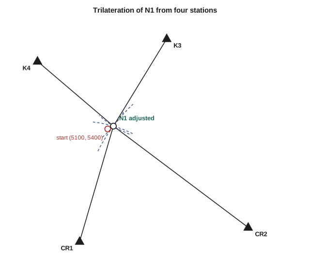
For the Oldman River bridge, Leah needs the coordinates of N1, a new control point on the east bank. She measures horizontal distances to N1 from four stations with known coordinates: pillars CR1 and CR2 and two existing control monuments, K3 and K4. All distances are reduced to grid. The distance standard deviation is 2 mm + 2 ppm, and the reference standard deviation is taken as 2 mm, so a short line has a weight close to one.
| Station | Easting (m) | Northing (m) | Measured distance to N1 (m) |
|---|---|---|---|
| CR1 | 5000.000 | 5000.000 | 427.2012 |
| CR2 | 5600.000 | 5050.000 | 599.8626 |
| K3 | 5310.000 | 5720.000 | 363.5561 |
| K4 | 4850.000 | 5640.000 | 354.8149 |
Worked problem
First iteration row for one distance
Start from approximate coordinates N1 = (5100.000, 5400.000), read roughly from a plan. Form the observation equation for the distance from CR1.
Show solution
- \[d^0 = \sqrt{(5100.000 - 5000.000)^2 + (5400.000 - 5000.000)^2} = 412.3106\ \text{m}\]
- \[\frac{\partial d}{\partial E} = \frac{100.000}{412.3106} = 0.2425, \qquad \frac{\partial d}{\partial N} = \frac{400.000}{412.3106} = 0.9701\]
- \[w = 427.2012 - 412.3106 = 14.8906\ \text{m}\]
- \[v_1 = 0.2425\,\delta E + 0.9701\,\delta N - 14.8906\]
Answer: The first row of A is [0.2425, 0.9701] and the first element of w is 14.8906 m. The other three rows are formed the same way, the normal equations are solved for δE and δN, and the process is repeated. The large misclosure, almost 15 m, shows that the starting point was poor, but it does not matter: the geometry is strong and the iteration will still converge.
def T(A): return [list(r) for r in zip(*A)]
def mul(A, B): return [[sum(a * b for a, b in zip(r, c)) for c in zip(*B)] for r in A]
def inv(A):
    n = len(A); M = [list(map(float, r)) + [1.0 if i == j else 0.0 for j in range(n)] for i, r in enumerate(A)]
    for c in range(n):
        p = max(range(c, n), key=lambda r: abs(M[r][c])); M[c], M[p] = M[p], M[c]
        d = M[c][c]; M[c] = [x / d for x in M[c]]
        for r in range(n):
            if r != c:
                f = M[r][c]; M[r] = [x - f * y for x, y in zip(M[r], M[c])]
    return [r[n:] for r in M]
def diag(v): return [[v[i] if i == j else 0.0 for j in range(len(v))] for i in range(len(v))]
def col(v): return [[x] for x in v]

# Trilateration of N1 by observation equations and Gauss-Newton iteration
import math

known = {'CR1': (5000.000, 5000.000), 'CR2': (5600.000, 5050.000),
         'K3': (5310.000, 5720.000), 'K4': (4850.000, 5640.000)}
obs = {'CR1': 427.2012, 'CR2': 599.8626, 'K3': 363.5561, 'K4': 354.8149}
s0 = 0.002                                     # reference standard deviation, m
sig = {k: 0.002 + 2e-6 * d for k, d in obs.items()}
P = diag([(s0 / sig[k]) ** 2 for k in obs])

E, N = 5100.0, 5400.0                          # approximate coordinates
for it in range(1, 10):
    A, w = [], []
    for k, d in obs.items():
        e, n = known[k]
        d0 = math.hypot(E - e, N - n)
        A.append([(E - e) / d0, (N - n) / d0])
        w.append([d - d0])
    Nm = mul(mul(T(A), P), A)
    Qxx = inv(Nm)
    dx = mul(Qxx, mul(mul(T(A), P), w))
    E, N = E + dx[0][0], N + dx[1][0]
    print(f"iteration {it}: dE = {dx[0][0]:+.4f}  dN = {dx[1][0]:+.4f}  ->  {E:.4f}, {N:.4f}")
    if abs(dx[0][0]) < 1e-5 and abs(dx[1][0]) < 1e-5:
        break

v = [mul([a], dx)[0][0] - wi[0] for a, wi in zip(A, w)]
r = len(obs) - 2
vtpv = sum(P[i][i] * v[i] ** 2 for i in range(len(v)))
s0_hat = math.sqrt(vtpv / r)
print("residuals (mm):", "  ".join(f"{k} {x * 1000:+.2f}" for k, x in zip(obs, v)))
print(f"a posteriori sigma0 = {s0_hat * 1000:.2f} mm (a priori {s0 * 1000:.1f} mm), {r} degrees of freedom")
print(f"sigma E = {s0 * math.sqrt(Qxx[0][0]) * 1000:.2f} mm, sigma N = {s0 * math.sqrt(Qxx[1][1]) * 1000:.2f} mm (a priori)")
print(f"correlation E,N = {Qxx[0][1] / math.sqrt(Qxx[0][0] * Qxx[1][1]):+.3f}")iteration 1: dE = +20.3122 dN = +9.9059 -> 5120.3122, 5409.9059 iteration 2: dE = -0.1728 dN = +0.0533 -> 5120.1394, 5409.9591 iteration 3: dE = +0.0000 dN = +0.0000 -> 5120.1395, 5409.9591 residuals (mm): CR1 -1.03 CR2 +1.33 K3 -0.93 K4 +0.71 a posteriori sigma0 = 0.99 mm (a priori 2.0 mm), 2 degrees of freedom sigma E = 2.32 mm, sigma N = 1.82 mm (a priori) correlation E,N = +0.088
The first iteration moves the point by about 20 m east and 10 m north, the second by less than 0.2 m, and the third by a few micrometres, after which the iteration stops. The adjusted position is 5120.1395 E, 5409.9591 N. The residuals are all about a millimetre, and the a posteriori reference standard deviation is about 1 mm, half the a priori 2 mm, which says that the distances were measured rather better than the specification. With only two degrees of freedom that estimate is too uncertain to justify rescaling, so the a priori standard deviations of about 2.3 mm in easting and 1.8 mm in northing are the ones to report.
Compare this with lesson 2, where the same point was set out by a single distance and azimuth from CR1 with standard deviations of about 6.0 mm and 3.2 mm. Four distances in a strong geometry give a point two to three times better, and, just as importantly, they give redundancy: if one distance had contained a blunder, the residuals would have revealed it.
Weights, units and scaling
In the program, the weight matrix uses the ratio of the reference standard deviation to each observation's standard deviation, so the weights are dimensionless and close to one. The cofactor matrix \(\mathbf{Q}_{xx}\) is then in units of the reference variance, and multiplying by \(\sigma_0^2\) gives covariances in square metres. Getting this bookkeeping right is the commonest source of wrong precisions in home-made adjustment programs. A good test is to scale every observation's standard deviation by the same factor: the adjusted coordinates must not change, and the a priori standard deviations must scale by exactly that factor.
Choosing approximate values
Gauss-Newton needs a start. For a level network the approximate heights can be anything, because the problem is linear. For a horizontal network they can usually be computed from a subset of the observations: a traverse or a chain of triangles run through the network without adjustment. Very poor starting values can cause slow convergence, convergence to a wrong solution where two circles intersect twice, or failure to converge at all. When the iteration diverges, the cause is far more often a blunder in the data, such as a wrong station name or a distance entered in feet instead of metres, than a mathematical failure, and checking the observations is the first step.
The iteration should stop when the corrections are small compared with the precision of the result, but it should always be run at least twice, so that the final residuals are computed with derivatives evaluated at the adjusted position. The residuals printed above come from the last iteration, where \(\delta\mathbf{x}\) is effectively zero, so \(\mathbf{v} = -\mathbf{w}\) and the residuals are simply the computed minus observed distances at the final coordinates.
What the software reports
Every adjustment report Leah will see from commercial software contains the same building blocks: the adjusted coordinates or heights, their standard deviations and often error ellipses, the residuals of every observation and their standardized values, the a posteriori reference variance with the number of degrees of freedom, and the result of a global statistical test. Understanding the observation equation method is what lets her read that report critically rather than accept it on trust. The next lessons look at a second way of setting up the adjustment, then apply observation equations to complete level and horizontal networks.
Common mistakes
MistakeForgetting to iterate a non-linear adjustment.
InsteadRepeat until corrections are negligible, recomputing A and w each time.
MistakeUsing degrees in angle derivatives.
InsteadUse radians for both the O − C values and the partial derivatives.
MistakeNot reducing angle misclosures to −π to π.
InsteadWrap the O − C of directions and angles to avoid full-circle jumps.
MistakeMixing units in the weight matrix.
InsteadExpress standard deviations in the same units as the observation equations.
MistakeBlaming the mathematics when iteration diverges.
InsteadCheck station names, units and blunders in the data first.
Summary and key terms
- Each observation gives one equation ℓ + v = F(x).
- Non-linear equations are linearized about approximate values; w is observed minus computed.
- The corrections are δx = (AᵀPA)⁻¹AᵀPw, and the process is iterated.
- Distance derivatives are the components of the unit vector between the points.
- Direction derivatives are ΔN/d² and −ΔE/d² in radians per metre.
- Redundancy n − u gives the degrees of freedom for the reference variance and testing.
- Four well-placed distances fix a point far better than a single distance and azimuth.
- Observation equation
- An equation expressing one observation as a function of the unknowns.
- Linearization
- Replacing a non-linear function by its first-order Taylor series about approximate values.
- Observed minus computed
- The difference between an observation and its value computed from approximate unknowns.
- Gauss-Newton method
- Iterative least squares in which the linearized problem is solved repeatedly.
- Trilateration
- Fixing positions from measured distances.
- Orientation unknown
- An extra unknown per set-up that relates measured directions to azimuths.
Practice problems
Work each problem on paper first, then reveal the answer to check.
How many unknowns and degrees of freedom are there when two new points are fixed by seven distances?
Show answer
Four unknowns and three degrees of freedom.
Give the partial derivatives of the distance from (100, 200) to an approximate point at (160, 280).
Show answer
d0 = 100; ∂d/∂E = 0.6, ∂d/∂N = 0.8.
For an azimuth to a point 500 m due north, what is ∂α/∂E?
Show answer
ΔN/d² = 500/250000 = 0.002 rad per m.
Why can a distance not control a point's position across the line?
Show answer
Its derivative across the line is zero.
An iteration moves a point by 2 m, then 0.02 m, then 0.00002 m. Has it converged?
Show answer
Yes; the last correction is negligible.
Lesson quiz · 5 questions
Score 60% or more to complete this lesson.
Create a free account to save your progress, take quizzes and earn a certificate.