Adjusting level networks

Level networks are the ideal place to put least squares into practice. The observation equations are linear, so there is no iteration; the weights follow a simple rule; and the results, a set of benchmark heights with standard deviations, are exactly what clients ask for. Yet level networks also show every important idea of network adjustment: the choice of datum, the difference between minimally and fully constrained adjustments, the use of residuals to judge the data, and the way precision depends on the network's shape. This lesson adjusts the Coulee Ridge benchmark network that lesson 6 treated by condition equations, this time by observation equations, and then uses it to check the published control.

Observation equations for levelled lines

A levelled line from benchmark \(i\) to benchmark \(j\) measures the height difference \(\Delta h_{ij} = H_j - H_i\). Its observation equation is

which is already linear in the unknown heights. In the design matrix, each row has +1 in the column of the forward benchmark, −1 in the column of the back benchmark, and zeros elsewhere. When one end is a fixed benchmark, its height is not an unknown, so it moves to the observation side: a line from fixed A to unknown P1 becomes \(\Delta h + H_A + v = H_{P1}\), and its row of \(\mathbf{A}\) has a single +1. Because every row contains only one or two non-zero entries, the design matrix of a large level network is mostly zeros, and professional software exploits that sparsity to adjust networks with thousands of benchmarks.

The weights are the reciprocals of the line lengths in kilometres, as lesson 3 explained, or of the number of set-ups in hilly terrain. If lines were levelled with different instruments or methods, such as a digital level with invar rods for some lines and a builder's level for others, each group needs its own standard deviation per root kilometre before the weights are formed.

Building the system

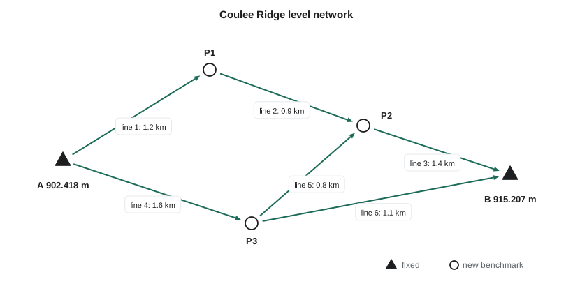
The network is the same as in lesson 6: six lines connect new benchmarks P1, P2 and P3 to the CGVD2013 benchmarks A (902.418 m) and B (915.207 m). The unknowns are the three new heights, so \(u = 3\), \(n = 6\) and \(r = 3\).

The columns correspond to P1, P2 and P3. Line 3 runs from P2 to the fixed benchmark B, so its equation is \(5.2748 + v_3 = 915.207 - H_{P2}\), which rearranges to \(5.2748 - 915.207 + v_3 = -H_{P2}\), giving the −1 in the P2 column. The weight matrix is \(\mathbf{P} = \mathrm{diag}(1/1.2,\ 1/0.9,\ 1/1.4,\ 1/1.6,\ 1/0.8,\ 1/1.1)\).

def T(A): return [list(r) for r in zip(*A)]
def mul(A, B): return [[sum(a * b for a, b in zip(r, c)) for c in zip(*B)] for r in A]
def inv(A):
    n = len(A); M = [list(map(float, r)) + [1.0 if i == j else 0.0 for j in range(n)] for i, r in enumerate(A)]
    for c in range(n):
        p = max(range(c, n), key=lambda r: abs(M[r][c])); M[c], M[p] = M[p], M[c]
        d = M[c][c]; M[c] = [x / d for x in M[c]]
        for r in range(n):
            if r != c:
                f = M[r][c]; M[r] = [x - f * y for x, y in zip(M[r], M[c])]
    return [r[n:] for r in M]
def diag(v): return [[v[i] if i == j else 0.0 for j in range(len(v))] for i in range(len(v))]
def col(v): return [[x] for x in v]

# Observation equation adjustment of the Coulee Ridge level network
import math

lines = [  # (from, to, observed rise in m, length in km)
    ('A', 'P1', 3.4126, 1.2), ('P1', 'P2', 4.1031, 0.9), ('P2', 'B', 5.2748, 1.4),
    ('A', 'P3', 6.8392, 1.6), ('P3', 'P2', 0.6773, 0.8), ('P3', 'B', 5.9493, 1.1)]

def adjust(fixed, unknown, s0=1.0):
    A, l = [], []
    for f, t, dh, K in lines:
        row, c = [0.0] * len(unknown), dh
        if f in unknown: row[unknown.index(f)] -= 1
        else: c += fixed[f]
        if t in unknown: row[unknown.index(t)] += 1
        else: c -= fixed[t]
        A.append(row); l.append([c])
    P = diag([1 / x[3] for x in lines])
    Qxx = inv(mul(mul(T(A), P), A))
    x = mul(Qxx, mul(mul(T(A), P), l))
    v = [mul([a], x)[0][0] - li[0] for a, li in zip(A, l)]
    r = len(lines) - len(unknown)
    vtpv = sum(P[i][i] * (v[i] * 1000) ** 2 for i in range(len(v)))
    return x, v, Qxx, r, vtpv

x, v, Q, r, vtpv = adjust({'A': 902.418, 'B': 915.207}, ['P1', 'P2', 'P3'])
print("fully constrained (A and B fixed)")
for i, name in enumerate(['P1', 'P2', 'P3']):
    print(f"  {name} = {x[i][0]:.4f} m   sigma = {math.sqrt(Q[i][i]):.2f} mm (a priori 1 mm/root km)")
print("  residuals (mm):", ", ".join(f"{t * 1000:+.2f}" for t in v))
print(f"  vTPv = {vtpv:.2f} mm^2, r = {r}, sigma0 = {math.sqrt(vtpv / r):.2f} mm/root km")

x2, v2, Q2, r2, vtpv2 = adjust({'A': 902.418}, ['P1', 'P2', 'P3', 'B'])
print("minimally constrained (A fixed only)")
print(f"  B adjusted = {x2[3][0]:.4f} m, published 915.2070, difference "
      f"{(x2[3][0] - 915.207) * 1000:+.1f} mm, sigma {math.sqrt(Q2[3][3]):.2f} mm")
print(f"  vTPv = {vtpv2:.2f} mm^2, r = {r2}, sigma0 = {math.sqrt(vtpv2 / r2):.2f} mm/root km")
print(f"  increase in vTPv from fixing B: {vtpv - vtpv2:.2f} mm^2")

fully constrained (A and B fixed)
  P1 = 905.8305 m   sigma = 0.83 mm (a priori 1 mm/root km)
  P2 = 909.9335 m   sigma = 0.73 mm (a priori 1 mm/root km)
  P3 = 909.2569 m   sigma = 0.68 mm (a priori 1 mm/root km)
  residuals (mm): -0.10, -0.07, -1.33, -0.27, -0.70, +0.77
  vTPv = 2.47 mm^2, r = 3, sigma0 = 0.91 mm/root km
minimally constrained (A fixed only)
  B adjusted = 915.2074 m, published 915.2070, difference +0.4 mm, sigma 1.23 mm
  vTPv = 2.38 mm^2, r = 2, sigma0 = 1.09 mm/root km
  increase in vTPv from fixing B: 0.10 mm^2

The fully constrained heights, 905.8305, 909.9335 and 909.2569 m, are identical to the condition adjustment of lesson 6, and so are the residuals. Their standard deviations, between about 0.7 and 0.8 mm, are smallest for P3, which is joined to both fixed benchmarks by relatively short lines, and largest for P1, which hangs off benchmark A by a single line on one side.

Choosing the datum

A levelled network measures only height differences. It fixes the shape of the height surface but not its vertical position, so at least one benchmark height must be held fixed to define the datum. An adjustment with exactly one fixed height is called minimally constrained. It allows the observations to fit together without any influence from the control, and its residuals and reference variance reflect only the quality of the levelling. An adjustment with two or more fixed heights is called fully constrained, or over-constrained. It forces the network to fit the published control, and its residuals reflect both the levelling and any inconsistency in the control.

Good practice is to run both. The minimally constrained adjustment comes first: if it shows a large reference variance or a large residual, the problem is in the field work. The fully constrained adjustment comes next: if it shows a substantially worse fit than the minimal one, the problem is in the control, and a published benchmark may have been disturbed, or its published height may come from an older adjustment.

For Coulee Ridge the comparison is reassuring. Holding A only, the adjusted height of B is 915.2074 m, just 0.4 mm from its published value and well within its standard deviation of 1.2 mm. The weighted sum of squared residuals rises only from 2.38 to 2.47 mm² when B is also held fixed, so the two benchmarks agree with each other, and the new levelling fits them both. Lesson 10 makes this kind of comparison into a formal statistical test.

Benchmark heights in Canada are now referred to CGVD2013, a geoid-based datum that replaced the levelling-based CGVD28 in 2013. Many older municipal benchmarks still carry CGVD28 heights, which differ from CGVD2013 by amounts that vary across the country. Mixing the two in a single adjustment would show up immediately as an inconsistency between fixed benchmarks, and the fully constrained adjustment would fail. Theo checks the datum and the publication date of every benchmark before it goes into an adjustment.

Weighting fixed benchmarks

Holding a benchmark absolutely fixed treats its published height as perfect. A more flexible approach treats the published height as an observation with its own standard deviation, so that the adjustment can move it slightly if the new levelling strongly disagrees. This is called a weighted constraint. With a very small standard deviation it behaves like a fixed point; with a large one it barely influences the result. Weighted constraints are useful when published heights come with their own standard deviations, as geodetic agency databases often provide, and they allow the new survey to be combined rigorously with the old one.

Specifications for levelling

Levelling specifications express the allowable misclosure of a loop or a line between benchmarks as \(k\sqrt{K}\) millimetres, where \(K\) is the length in kilometres and \(k\) depends on the order or class of the work. Canadian federal specifications and provincial standards set tolerances of a few millimetres per root kilometre for the highest orders, rising for lower-order work, and municipal engineering standards for subdivisions are normally set in the same form. Coulee Geomatics' project specification for Coulee Ridge allowed 8 mm√K for loop closures; the worst loop, P3 to P2 to B, 3.3 km long, closed to 2.8 mm against an allowance of 14.5 mm.

A misclosure check like this is a test of the raw data before adjustment. The adjustment adds two things that the check cannot give: the best heights from all lines together, and a standard deviation for each height. Specifications increasingly state their requirements in terms of the adjusted results, for example that every new benchmark must have a standard deviation below a stated value relative to the nearest control, which can only be verified from the adjustment.

Reading the residuals

The residuals of a well-behaved level adjustment are small, show no pattern, and are roughly proportional to the square root of the line lengths. Patterns are diagnostic. If all lines run uphill have negative residuals and all lines run downhill have positive ones, the rods may have a scale error or the level may have a collimation error that was not cancelled. If the residuals of lines levelled on one particular day are all large, something went wrong that day: a disturbed turning point, a heat-affected instrument, a misread rod. If a single residual is far larger than the others, it may be a blunder, though as lesson 4 warned, least squares can spread a blunder among several lines. Lesson 10 explains how to test residuals properly, taking into account that lines in weakly connected parts of the network have less ability to reveal their own errors.

Network shape and precision

The precision of an adjusted benchmark depends on the network as well as the levelling. A benchmark at the end of a single spur line, with no second connection, has no redundancy at all: its height is whatever that line says, its residual is always zero, and a blunder in that line can never be detected. A benchmark in the middle of a well-connected mesh, joined by several short lines to points that are themselves well determined, has a small standard deviation and strong checks. Designing level networks so that every new benchmark lies on at least one loop, and preferably on two, is the simplest rule of good network design, and lesson 11 shows how to quantify it before going to the field.