Sequential and Kalman estimation

All of the adjustments so far have been batch adjustments: collect every observation, then solve once. Many geomatics problems do not work that way. Observations arrive over time, from a GNSS receiver every second, a monitoring prism every hour, or a new level line added to a network that was adjusted last year, and the user wants an up-to-date estimate after each one without recomputing everything from scratch. When the unknowns stay fixed, the tool is sequential least squares. When the unknowns themselves change with time, as a moving vehicle's position does or a slowly sliding retaining wall's displacement does, the tool is the Kalman filter. Both are least squares in disguise, and this final lesson shows how they follow from what has come before.

Sequential least squares

Suppose a batch adjustment of a first group of observations has produced estimates \(\hat{\mathbf{x}}_1\) with cofactor matrix \(\mathbf{Q}_1\). A second group of observations arrives, with design matrix \(\mathbf{A}_2\), observations \(\boldsymbol{\ell}_2\) and cofactor matrix \(\mathbf{R}_2\), uncorrelated with the first group. The combined least squares solution can be computed by updating the first solution rather than starting again:

The bracket \(\boldsymbol{\ell}_2 - \mathbf{A}_2\hat{\mathbf{x}}_1\) is the innovation: the difference between what the new observations say and what the current estimate predicted they would say. The matrix \(\mathbf{K}\) is the gain, which decides how much the estimate moves in response. A precise new observation (small \(\mathbf{R}_2\)) of a poorly known quantity (large \(\mathbf{Q}_1\)) gets a large gain and moves the estimate a lot; an imprecise observation of a well-known quantity barely moves it. The matrix to invert has the size of the new group, not of the whole network, which is the computational saving.

The result is exactly the same as a batch adjustment of all observations together, not an approximation. The innovation also gives a natural test: its standardized value tells whether the new observations agree with the old solution, and a large value flags either a blunder in the new data or a change in the network, such as a disturbed benchmark.

def T(A): return [list(r) for r in zip(*A)]
def mul(A, B): return [[sum(a * b for a, b in zip(r, c)) for c in zip(*B)] for r in A]
def inv(A):
    n = len(A); M = [list(map(float, r)) + [1.0 if i == j else 0.0 for j in range(n)] for i, r in enumerate(A)]
    for c in range(n):
        p = max(range(c, n), key=lambda r: abs(M[r][c])); M[c], M[p] = M[p], M[c]
        d = M[c][c]; M[c] = [x / d for x in M[c]]
        for r in range(n):
            if r != c:
                f = M[r][c]; M[r] = [x - f * y for x, y in zip(M[r], M[c])]
    return [r[n:] for r in M]
def diag(v): return [[v[i] if i == j else 0.0 for j in range(len(v))] for i in range(len(v))]
def col(v): return [[x] for x in v]
# Sequential least squares: add a new level line without readjusting from scratch
import math

HA, HB = 902.418, 915.207
def row(f, t, dh, K):                     # unknowns P1, P2, P3
    idx = {'P1': 0, 'P2': 1, 'P3': 2}; r, c = [0.0] * 3, dh
    if f in idx: r[idx[f]] -= 1
    else: c += {'A': HA, 'B': HB}[f]
    if t in idx: r[idx[t]] += 1
    else: c -= {'A': HA, 'B': HB}[t]
    return r, c, K

first = [('A', 'P1', 3.4126, 1.2), ('P1', 'P2', 4.1031, 0.9), ('P2', 'B', 5.2748, 1.4),
         ('A', 'P3', 6.8392, 1.6), ('P3', 'P2', 0.6773, 0.8)]
new = ('P3', 'B', 5.9493, 1.1)

def batch(lines):
    R = [row(*x) for x in lines]
    A = [r for r, _, _ in R]; l = col([c for _, c, _ in R]); P = diag([1 / K for _, _, K in R])
    Q = inv(mul(mul(T(A), P), A))
    return mul(Q, mul(mul(T(A), P), l)), Q

x, Q = batch(first)
print("after the first five lines: ", "  ".join(f"{v[0]:.4f}" for v in x))

# Update with the sixth line: x+ = x + K (l2 - A2 x),  K = Q A2^T (R2 + A2 Q A2^T)^-1
a2, l2, K2 = row(*new)
A2 = [a2]
S = mul(mul(A2, Q), T(A2))[0][0] + K2           # innovation cofactor
G = [[g[0] / S] for g in mul(Q, T(A2))]          # gain (3 x 1)
innov = l2 - mul(A2, x)[0][0]
x = [[x[i][0] + G[i][0] * innov] for i in range(3)]
GA = mul(G, A2)
Q = mul([[(1.0 if i == j else 0.0) - GA[i][j] for j in range(3)] for i in range(3)], Q)
print(f"innovation of the new line = {innov * 1000:+.2f} mm, its standardized value = {innov / math.sqrt(S) * 1000:+.2f}")
print("after sequential update:    ", "  ".join(f"{v[0]:.4f}" for v in x))
xb, Qb = batch(first + [new])
print("batch with all six lines:   ", "  ".join(f"{v[0]:.4f}" for v in xb))
print("sigma (mm), sequential vs batch:",
      "  ".join(f"{math.sqrt(Q[i][i]):.3f}/{math.sqrt(Qb[i][i]):.3f}" for i in range(3)))

after the first five lines:  905.8303  909.9332  909.2564
innovation of the new line = -1.34 mm, its standardized value = -0.97
after sequential update:     905.8305  909.9335  909.2569
batch with all six lines:    905.8305  909.9335  909.2569
sigma (mm), sequential vs batch: 0.829/0.829  0.729/0.729  0.683/0.683

The sequential update reproduces the batch heights and standard deviations of lesson 7 exactly. The innovation of the new line is −1.34 mm, with a standardized value of about −1, so the new line agrees well with the first five and there is no sign of a problem. Had the standardized innovation been 4 or 5, Leah would have checked the new line's field notes and whether any benchmark had been disturbed between the two campaigns.

From fixed to moving unknowns

Sequential least squares assumes that the unknowns do not change. In deformation monitoring and navigation they do. A monitoring point on a retaining wall moves slowly as the soil behind it creeps; a vehicle's position changes every fraction of a second. Each new observation then refers to a different state of the system, and the estimator must account for how the state evolves between observations. The Kalman filter, published by Rudolf Kálmán in 1960 and used within a decade for spacecraft navigation, does this by combining two sources of information at every step: a dynamic model that predicts how the state changes, and the new observations.

The Kalman filter

The state vector \(\mathbf{x}_k\) at epoch \(k\) contains everything needed to describe the system, for example a position and a velocity. The dynamic model predicts the next state from the current one:

where \(\mathbf{F}\) is the transition matrix and \(\mathbf{u}_k\) is process noise, with covariance \(\mathbf{Q}_p\), which represents everything the model does not capture, such as small accelerations. The observations relate to the state through \(\mathbf{z}_k = \mathbf{H}\mathbf{x}_k + \mathbf{e}_k\), with measurement noise covariance \(\mathbf{R}\). The filter then alternates between two steps.

The prediction step projects the previous estimate forward in time and enlarges its covariance to reflect the process noise:

The update step corrects the prediction with the new observation, using exactly the sequential least squares formulas with the prediction as the prior:

If the process noise were zero, the filter would reduce to sequential least squares, treating the state as fixed. With process noise, older observations gradually lose influence, so the filter can follow genuine changes. The choice of \(\mathbf{Q}_p\) is the main tuning decision. Too small, and the filter is sluggish, believing its model over the data and responding late to real movement. Too large, and it chases measurement noise, producing a jumpy estimate and false alarms.

A constant-velocity model

For a monitoring point moving along one direction, a simple and widely used model has two states: the displacement \(x\) and the velocity \(\dot{x}\). Over an interval \(\Delta t\), with velocity treated as roughly constant but allowed to drift by process noise,

where \(q\) is the spectral density of the velocity random walk. The observation is the measured displacement only; the velocity is never measured directly but is estimated from how displacements change over time. That is one of the filter's chief strengths in monitoring: a velocity with a standard deviation is exactly what an engineer needs to decide whether a structure is accelerating.

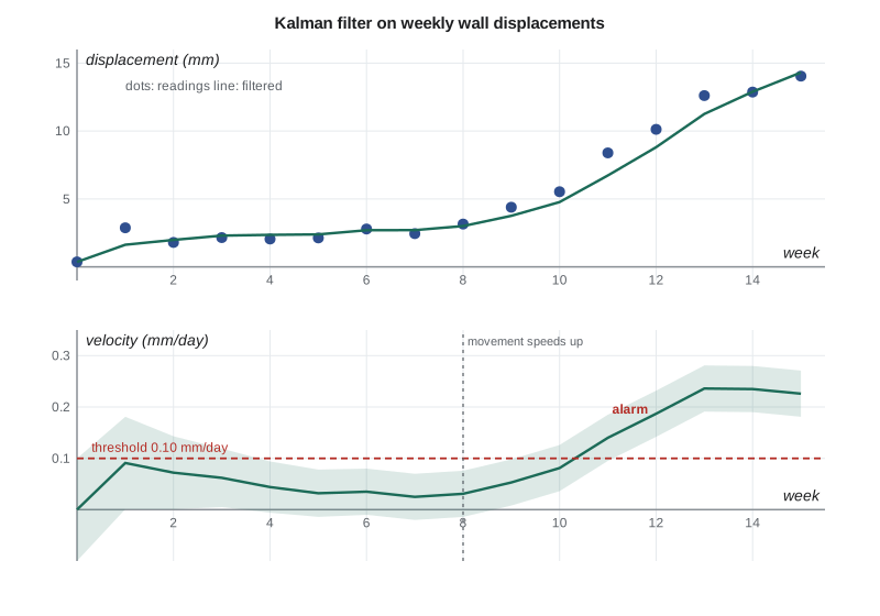
Coulee Geomatics monitors a retaining wall along a road cut above the Oldman River valley, where a slope failure two years ago led the municipality to rebuild the wall. An automated total station on a stable pillar measures prisms on the wall each week, and the offsets perpendicular to the wall are reduced to displacement since the baseline survey. The geotechnical engineer has set a review threshold of 0.10 mm per day of outward movement.

def T(A): return [list(r) for r in zip(*A)]
def mul(A, B): return [[sum(a * b for a, b in zip(r, c)) for c in zip(*B)] for r in A]
def inv(A):
    n = len(A); M = [list(map(float, r)) + [1.0 if i == j else 0.0 for j in range(n)] for i, r in enumerate(A)]
    for c in range(n):
        p = max(range(c, n), key=lambda r: abs(M[r][c])); M[c], M[p] = M[p], M[c]
        d = M[c][c]; M[c] = [x / d for x in M[c]]
        for r in range(n):
            if r != c:
                f = M[r][c]; M[r] = [x - f * y for x, y in zip(M[r], M[c])]
    return [r[n:] for r in M]
def diag(v): return [[v[i] if i == j else 0.0 for j in range(len(v))] for i in range(len(v))]
def col(v): return [[x] for x in v]
# Constant-velocity Kalman filter for a retaining wall monitoring prism
import math, random

random.seed(8)
dt = 7.0                                   # days between epochs
sig_meas = 1.0                             # mm, total station precision for the offset
q = 0.0001                                 # process noise: velocity random walk, (mm/day)^2 per day
truth, obs, x_true, v_true = [], [], 0.0, 0.05
for k in range(16):
    if k == 8:
        v_true = 0.20                      # movement speeds up after the spring thaw
    if k > 0:
        x_true += v_true * dt
    truth.append(x_true)
    obs.append(x_true + random.gauss(0, sig_meas))

F = [[1.0, dt], [0.0, 1.0]]
Qp = [[q * dt ** 3 / 3, q * dt ** 2 / 2], [q * dt ** 2 / 2, q * dt]]
H = [[1.0, 0.0]]
R = [[sig_meas ** 2]]
x = [[obs[0]], [0.0]]                      # start: first reading, zero velocity
P = [[sig_meas ** 2, 0.0], [0.0, 0.1 ** 2]]
ALARM = 0.10                               # mm/day
print(" week   obs mm   filt mm   vel mm/day   sigma vel   status")
for k, z in enumerate(obs):
    if k > 0:                              # predict
        x = mul(F, x)
        P = [[a + b for a, b in zip(r1, r2)] for r1, r2 in zip(mul(mul(F, P), T(F)), Qp)]
    S = mul(mul(H, P), T(H))[0][0] + R[0][0]
    K = [[r[0] / S] for r in mul(P, T(H))]  # gain
    innov = z - x[0][0]
    x = [[x[0][0] + K[0][0] * innov], [x[1][0] + K[1][0] * innov]]
    KH = mul(K, H)
    P = mul([[(1.0 if i == j else 0.0) - KH[i][j] for j in range(2)] for i in range(2)], P)
    vel, sv = x[1][0], math.sqrt(P[1][1])
    status = "ALARM" if vel - 1.645 * sv > ALARM else ("watch" if vel > ALARM else "ok")
    print(f"{k:>5}{z:>9.2f}{x[0][0]:>10.2f}{vel:>12.3f}{sv:>12.3f}   {status}")
print(f"true displacement after 15 weeks = {truth[-1]:.2f} mm")

 week   obs mm   filt mm   vel mm/day   sigma vel   status
    0     0.37      0.37       0.000       0.100   ok
    1     2.88      1.63       0.091       0.090   ok
    2     1.80      1.99       0.072       0.071   ok
    3     2.16      2.30       0.062       0.057   ok
    4     2.05      2.36       0.044       0.050   ok
    5     2.13      2.39       0.032       0.046   ok
    6     2.79      2.70       0.035       0.045   ok
    7     2.45      2.71       0.025       0.045   ok
    8     3.15      3.01       0.031       0.045   ok
    9     4.39      3.76       0.053       0.045   ok
   10     5.53      4.77       0.081       0.045   ok
   11     8.39      6.73       0.140       0.045   watch
   12    10.12      8.81       0.187       0.045   ALARM
   13    12.61     11.26       0.236       0.045   ALARM
   14    12.87     12.89       0.235       0.045   ALARM
   15    14.04     14.31       0.226       0.045   ALARM
true displacement after 15 weeks = 13.65 mm

The simulated wall creeps at 0.05 mm per day for the first eight weeks and then, after the spring thaw, at 0.20 mm per day. The individual readings scatter by about a millimetre, so week-to-week differences are useless for judging speed: a 1 mm error in two readings a week apart corresponds to a velocity error of about 0.2 mm per day. The filter's velocity estimate settles to between about 0.025 and 0.055 mm per day from week 4 to week 9, with a standard deviation of 0.045 mm per day. After the movement speeds up, the estimate climbs over the next few weeks, crosses the 0.10 mm per day threshold at week 11, and by week 12 is above the threshold by more than 1.645 standard deviations, which the program treats as a confident exceedance and labels as an alarm. By the end it reads about 0.23 mm per day, close to the true 0.20.

The delay between the change at week 8 and the alarm at week 12 is the price of smoothing. A larger process noise would respond sooner but would also have raised the velocity above the threshold several times during the slow phase on noise alone. Choosing the process noise is therefore a decision with engineering consequences, made with the geotechnical engineer, and tested on historical data before the system goes live. More frequent readings shorten the delay, which is one reason automated monitoring systems read hourly rather than weekly.

Kalman filters elsewhere in geomatics

The same framework runs inside many instruments surveyors use every day. An RTK GNSS receiver uses a Kalman filter to estimate position, receiver clock and carrier phase ambiguities from each epoch of observations. GNSS and inertial navigation systems on mobile mapping vehicles and lidar aircraft are integrated by Kalman filters that blend high-rate inertial measurements with lower-rate GNSS fixes, so the trajectory stays smooth and survives short satellite outages under bridges or trees. Precise point positioning services, machine control on earthmoving equipment, and robotic total stations tracking a moving prism all depend on recursive estimation of this kind. GEOM-300 returns to the filter in the context of GNSS and inertial integration.

A related technique, the smoother, runs a filter forwards and then backwards through the data after the fact, so that each estimate uses future as well as past observations. Post-processed mobile mapping trajectories are computed this way, and in monitoring the smoothed velocity history gives the clearest picture of when movement actually began.

Bringing the course together

Every topic in this course comes back to a few ideas. Measurements have errors whose statistics can be described (lesson 1) and propagated (lesson 2). Weights express the relative precision of observations (lesson 3). The least squares principle chooses the most probable consistent solution (lesson 4), whether expressed through observation equations (lesson 5) or condition equations (lesson 6), and it applies equally to level networks (lesson 7) and horizontal networks (lesson 8). The covariance matrix it produces describes precision, drawn as error ellipses (lesson 9). Statistical tests check that the solution and its stated precision can be trusted (lesson 10). Pre-analysis designs surveys before they are measured (lesson 11). And sequential and Kalman estimation extend the same ideas to data that arrive over time. Leah now has the tools to read any adjustment report critically and to write one that Ruth will be prepared to sign.