
GEOM-220 · Lesson 1 of 12 · 23 min
Measurement errors and statistics
No measurement is exact. A total station that reports a distance of 427.200 m is giving its best estimate of a quantity whose true value nobody knows, and if the same line is measured ten times the instrument will report ten slightly different numbers. Geomatics engineers do not treat this as a nuisance to be hidden. They treat it as information. Knowing how large and how well behaved the errors are is what allows a surveyor to say that a boundary corner is correct to 2 cm, that a bridge pier has moved by 6 mm, or that a new benchmark is good enough to be published. This course, GEOM-220 Adjustment of Observations, is about that knowledge: how to describe errors, how they carry into computed results, and how to combine redundant measurements by least squares so that the answer is both the most probable one and accompanied by an honest statement of its quality.
Throughout the course we follow Coulee Geomatics in Lethbridge, the firm met in CIV-250 and GEOM-200. Ruth Albrecht, ALS, P.Eng., runs the survey department. Theo Martel is the technologist who looks after control networks and adjustment software, and Leah Tran is the co-op student who has just been handed her first set of raw field files. Over twelve lessons Leah will adjust a benchmark network for the Coulee Ridge subdivision, a control network for the Oldman River bridge, a pipeline GNSS network and a monitoring scheme for a retaining wall. This first lesson covers the vocabulary and statistics on which everything else rests.
Three kinds of error
Every difference between a measured value and the true value can be traced to one of three causes, and each is handled differently.
A blunder, sometimes called a gross error or a mistake, is a human or procedural failure: reading 1.583 m on a levelling rod as 1.538 m, sighting the wrong prism, entering an instrument height of 1.55 m as 15.5 m, or occupying the wrong monument. Blunders are not small and they do not follow any statistical pattern. No amount of averaging removes them. They are prevented by careful procedure, caught by independent checks and, as lesson 10 will show, detected by statistical testing of redundant observations. A survey without redundancy can contain a blunder that nobody ever notices.
A systematic error follows a physical law or a fixed pattern, so it has the same sign and a predictable size under the same conditions. Examples include a steel tape that is 4 mm too long, an EDM reflector constant entered incorrectly, a level whose line of sight tilts slightly, atmospheric refraction, and the effect of temperature on the speed of light. Systematic errors do not shrink when a measurement is repeated, because every repetition is biased in the same way. They are removed by calibration, by applying corrections computed from a model, or by field procedures that make them cancel, such as balancing backsight and foresight lengths in levelling or measuring angles on both faces of a total station.
A random error is what is left once blunders have been eliminated and systematic errors corrected. Random errors come from the many small, unpredictable influences on a measurement: the observer's eye, slight vibration of the tripod, shimmering air, the last digit of the display. Individually they are unpredictable, but as a group they follow well-defined statistical laws. Small errors are more common than large ones, positive and negative errors are equally likely, and very large random errors are very rare. Least squares adjustment is designed for random errors. It assumes that blunders have been found and systematic effects modelled, and it then distributes the remaining random errors in the most probable way.
| Kind | Behaviour | How it is handled |
|---|---|---|
| Blunder | Large, irregular, often a single observation | Procedure, independent checks, redundancy and statistical testing |
| Systematic | Same sign and predictable size under the same conditions | Calibration, corrections from a model, balanced field procedures |
| Random | Small, equally likely positive or negative, follows probability laws | Repetition, redundancy and least squares adjustment |
Precision and accuracy
Two words are used constantly, and they mean different things. Precision describes how closely repeated measurements agree with each other. Accuracy describes how closely a measurement, or the mean of a set of measurements, agrees with the true value. A set of measurements can be precise without being accurate if a systematic error shifts all of them together: an EDM with the wrong prism constant may repeat a distance to within a millimetre every time and still be 30 mm wrong. A set can also be accurate on average but imprecise, scattered widely about the true value.
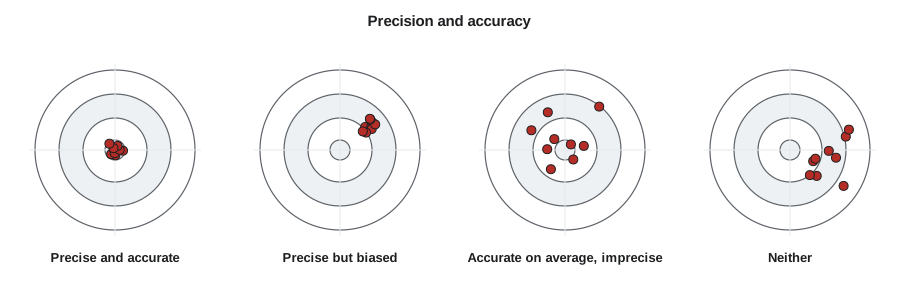
In practice, precision is easy to estimate from the measurements themselves, while accuracy can only be assessed by comparing with something independent and better: a calibration baseline, a published control point, or a measurement made by a superior method. For this reason survey specifications usually state both an internal precision requirement, checked by the adjustment, and an accuracy check against existing control.
Describing a set of repeated measurements
Suppose Leah measures the same distance \(n\) times and obtains values \(x_1, x_2, \ldots, x_n\). The best estimate of the distance is the arithmetic mean:
The difference between each measurement and the mean is called a residual, \(v_i = \bar{x} - x_i\). Residuals always sum to zero when the mean is used. The spread of the measurements is described by the sample standard deviation:
The divisor is \(n - 1\) rather than \(n\) because one degree of freedom has been used up in computing the mean from the same data. With only one measurement there is no information about spread at all; with two there is one degree of freedom, and so on. This idea, that each estimated quantity consumes one degree of freedom and that only the remaining redundancy tells us about precision, is the seed of every least squares adjustment in this course.
The standard deviation describes a single measurement. The mean of \(n\) measurements is more precise than any one of them, and its standard error is:
Doubling the precision of a mean therefore requires four times as many measurements. This square-root law explains why survey crews repeat measurements a handful of times rather than dozens: beyond four to eight repetitions the gain is small compared with the cost, and remaining systematic errors soon dominate.
The variance is the square of the standard deviation, \(s^2\) or, for the theoretical value, \(\sigma^2\). Variances are awkward to read because their units are squared (mm² for a distance), but they are what the mathematics works with, because variances of independent quantities add while standard deviations do not.
The normal distribution
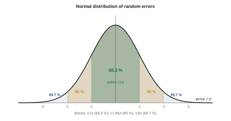
Random errors in surveying measurements are very closely described by the normal, or Gaussian, distribution. Its bell-shaped probability curve is completely defined by its mean and standard deviation. Several facts about it are used every day.
| Interval | Probability of a random error falling inside | Common name |
|---|---|---|
| ±1σ | 68.3 % | Standard error, one sigma |
| ±1.645σ | 90 % | 90 per cent confidence |
| ±1.96σ | 95 % | 95 per cent confidence, used in most accuracy standards |
| ±2.576σ | 99 % | 99 per cent confidence |
| ±3σ | 99.7 % | Often used as a rejection limit for outliers |
These numbers apply to a single quantity such as a distance or a height. For a two-dimensional position the probabilities are different, because the error can fall anywhere in a plane: a circle of radius one standard deviation contains only about 39 per cent of errors, not 68 per cent. Lesson 9 explains how error ellipses deal with this, and why the 95 per cent multiplier for a horizontal position is 2.448 instead of 1.96.
Accuracy standards in North America are almost always stated at the 95 per cent confidence level. The Geodetic Survey of Canada's accuracy standards for positioning define network and local accuracy at 95 per cent, and provincial survey standards, such as the Alberta Land Surveyors' Association Manual of Standard Practice, express their required accuracies in the same way. When a specification says that control must be good to 2 cm at 95 per cent, it means that the 95 per cent interval, about two standard deviations, must be no wider than 2 cm.
Confidence intervals for the mean
With a large number of measurements, the 95 per cent confidence interval for the true value is \(\bar{x} \pm 1.96\, s_{\bar{x}}\). With few measurements, the standard deviation is itself uncertain, and the multiplier must be taken from Student's t distribution instead. For example, with five measurements (four degrees of freedom) the 95 per cent t value is 2.776, considerably more than 1.96, and with ten measurements (nine degrees of freedom) it is 2.262. Survey software that reports a 95 per cent interval from a handful of observations should be using these larger values.
Finding outliers in repeated measurements
Before computing a mean, a careful surveyor looks at the data. A value far from the others may be a blunder. A simple rule rejects any residual larger than three standard deviations, although with small samples the standard deviation is inflated by the outlier itself, so the outlier can hide. More formal tests, and the methods used inside adjustments, are covered in lesson 10. For now the rule is: never delete a measurement simply because it is inconvenient. Look for a reason, such as a note in the field book, a wrong prism or a misread rod, and if none can be found, remeasure.
Worked problem
Repeated distances on a calibration baseline
Before starting the bridge control survey, Leah measures the 427 m line between two pillars ten times with the firm's total station. The values, in metres, are 427.2031, 427.2006, 427.2022, 427.1995, 427.2014, 427.2027, 427.2009, 427.2018, 427.2041 and 427.2003. Find the mean, the standard deviation of one measurement, the standard error of the mean and the 95 per cent confidence interval.
Show solution
- \[\bar{x} = \frac{4272.0166}{10} = 427.20166\ \text{m}\]
- Residuals in millimetres range from −2.4 mm (for 427.2041) to +2.2 mm (for 427.1995). Their squares sum to about 17.6 mm².
- \[s = \sqrt{\frac{17.6}{9}} = 1.40\ \text{mm}\]
- \[s_{\bar{x}} = \frac{1.40}{\sqrt{10}} = 0.44\ \text{mm}\]
- \[\text{95 per cent interval} = 427.2017 \pm 2.262 \times 0.00044 = 427.2017 \pm 0.0010\ \text{m}\]
Answer: The mean is 427.2017 m with a standard error of about 0.4 mm. A single measurement has a standard deviation of about 1.4 mm, which agrees with the instrument's specification for a line of this length. The mean is precise, but it is only accurate if the instrument's constant and scale have been calibrated; lesson 4 shows how a calibration baseline is used to find them.
# Statistics of ten repeated distance measurements
import math

d = [427.2031, 427.2006, 427.2022, 427.1995, 427.2014,
     427.2027, 427.2009, 427.2018, 427.2041, 427.2003]
n = len(d)
mean = sum(d) / n
v = [mean - x for x in d]                       # residuals
s = math.sqrt(sum(r * r for r in v) / (n - 1))  # one measurement
se = s / math.sqrt(n)                           # the mean
t95 = {4: 2.776, 9: 2.262, 19: 2.093, 1000: 1.960}[n - 1]   # Student's t, 95 per cent, approximate table

print(f"n = {n}, mean = {mean:.5f} m")
print(f"sum of residuals = {sum(v) * 1000:.3f} mm (always zero)")
print(f"standard deviation of one measurement s = {s * 1000:.2f} mm")
print(f"standard error of the mean = {se * 1000:.2f} mm")
print(f"95 per cent interval: {mean:.4f} +/- {t95 * se:.4f} m (t = {t95})")
print(f"largest residual = {max(abs(r) for r in v) * 1000:.1f} mm = {max(abs(r) for r in v) / s:.2f} s")
flag = [x for x, r in zip(d, v) if abs(r) > 3 * s]
print("values beyond 3 s:", flag if flag else "none")

# The square-root law: how many repetitions for a given precision of the mean?
for target in (1.0, 0.5, 0.25):
    reps = math.ceil((s * 1000 / target) ** 2)
print(f"for a standard error of {target} mm you need about {reps} measurements")n = 10, mean = 427.20166 m sum of residuals = 0.000 mm (always zero) standard deviation of one measurement s = 1.40 mm standard error of the mean = 0.44 mm 95 per cent interval: 427.2017 +/- 0.0010 m (t = 2.262) largest residual = 2.4 mm = 1.74 s values beyond 3 s: none for a standard error of 1.0 mm you need about 2 measurements for a standard error of 0.5 mm you need about 8 measurements for a standard error of 0.25 mm you need about 32 measurements
The program confirms the hand calculation and adds two useful facts. The largest residual is only about 1.7 standard deviations, so there is no reason to suspect a blunder. And the square-root law shows how expensive extra precision is: halving the standard error of the mean from 1 mm to 0.5 mm needs about four times as many measurements, from 2 to 8, and halving it again to 0.25 mm needs about 32. In practice, beyond a few repetitions, the remaining systematic errors, such as an imperfectly known prism constant or atmospheric correction, will dominate long before random error does.
Covariance and correlation
When two or more quantities are estimated from the same measurements, their errors are often related. The easting and northing of a point fixed by a single distance and azimuth are an example: an error in the azimuth moves the point sideways, changing both coordinates together. The covariance \(\sigma_{xy}\) measures how two quantities vary together, and the correlation coefficient \(\rho = \sigma_{xy} / (\sigma_x \sigma_y)\) expresses it on a scale from −1 to +1. Variances and covariances are collected into a covariance matrix:
The covariance matrix is the central object of this course. Lesson 2 shows how it propagates through computations, lesson 3 how its inverse gives the weights, lesson 5 how least squares produces it for the adjusted unknowns, and lesson 9 how it is drawn as an error ellipse. Raw field observations are usually treated as uncorrelated, so their covariance matrix is diagonal, but computed quantities such as coordinates almost never are.
A note on rounding and significant figures
Field software often reports more digits than the measurement deserves, and adjustment software carries even more internally. Two habits keep things honest. First, carry plenty of digits during computation, because rounding intermediate results adds avoidable error. Second, report results to a number of digits that reflects their precision: a coordinate with a standard error of 5 mm should be reported to the millimetre, not to a tenth of a millimetre, and its standard error to two significant figures at most. A table of adjusted coordinates to the micrometre suggests a precision that the survey did not achieve.
Common mistakes
MistakeTreating precision as accuracy.
InsteadRemember that tight agreement between repeated measurements says nothing about systematic errors; check against independent control or a calibration.
MistakeAveraging to remove a blunder.
InsteadFind and remove blunders by checks and testing; averaging only spreads them into the result.
MistakeDividing by n instead of n − 1 for a sample standard deviation.
InsteadUse n − 1, because the mean was computed from the same data.
MistakeUsing 1.96 for a 95 per cent interval from five measurements.
InsteadUse Student's t (2.776 for four degrees of freedom) when the sample is small.
MistakeApplying single-quantity probabilities to a 2D position.
InsteadUse error ellipse multipliers for positions (lesson 9).
Summary and key terms
- Errors are blunders, systematic errors or random errors, and each is handled differently.
- Precision is agreement between repeated measurements; accuracy is closeness to the true value.
- The mean is the best estimate from repeated measurements; s uses n − 1 degrees of freedom.
- The standard error of the mean is s/√n, so precision improves only with the square root of the number of repetitions.
- About 68 per cent of random errors fall within ±1σ and 95 per cent within ±1.96σ for a single quantity.
- Most North American accuracy standards are stated at 95 per cent confidence.
- The covariance matrix describes the precision of several quantities and how their errors are related.
- Blunder
- A mistake or gross error that does not follow statistical laws.
- Systematic error
- An error that follows a physical law or fixed pattern and has a predictable size and sign.
- Random error
- A small, unpredictable error that follows probability laws.
- Precision
- The closeness of repeated measurements to one another.
- Accuracy
- The closeness of a measurement or estimate to the true value.
- Residual
- The difference between an estimated value and an individual measurement.
- Standard error
- The standard deviation of an estimated quantity such as a mean.
- Degrees of freedom
- The number of observations in excess of the minimum needed, which carries information about precision.
- Covariance matrix
- A square matrix of variances and covariances describing the precision of several quantities.
Practice problems
Work each problem on paper first, then reveal the answer to check.
A height difference is measured six times with a standard deviation of 1.2 mm per measurement. What is the standard error of the mean?
Show answer
\(1.2/\sqrt{6} = 0.49\) mm.
Classify: a level whose line of sight tilts by 10 seconds.
Show answer
Systematic error (collimation); removed by balancing sight lengths or calibration.
Within what interval would 95 per cent of single measurements fall if σ = 3 mm?
Show answer
±1.96 × 3 = ±5.9 mm.
Four measurements of an angle give a standard deviation of 4″. What is the 95 per cent interval for the mean using Student's t for three degrees of freedom (3.182)?
Show answer
\(\pm 3.182 \times 4/\sqrt{4} = \pm 6.4''\).
Two quantities have σx = 4 mm, σy = 5 mm and σxy = 10 mm². What is their correlation coefficient?
Show answer
\(10/(4 \times 5) = 0.5\).
Lesson quiz · 5 questions
Score 60% or more to complete this lesson.
Create a free account to save your progress, take quizzes and earn a certificate.