Error propagation

Surveyors rarely want the raw measurements themselves. They want coordinates, areas, elevations, volumes and offsets that are computed from those measurements, and every computed quantity inherits the uncertainty of the numbers that went into it. Error propagation is the set of rules that tells us how much. Given the standard deviations, and if necessary the covariances, of the measured quantities, it gives the standard deviations and covariances of anything computed from them. It is the most widely used tool in this course, because it answers the questions engineers ask before, during and after every survey: will this instrument and procedure meet the specification, how precise is the stake-out of this pier, how much of the uncertainty in a volume comes from the cross-sections and how much from the station spacing?

In this lesson Leah Tran is setting out the first new control point, N1, for the bridge network from pillar CR1 by a single distance and azimuth. Theo Martel asks her a simple question before she goes to the field: if the total station measures distances to 2 mm + 2 ppm and directions to 3 seconds, how well will N1's coordinates be known? Answering it needs the general law of propagation of variances.

Linear functions of one quantity

The simplest case is a quantity \(y\) computed from one measurement \(x\) by multiplying by a constant: \(y = a x\). If \(x\) has standard deviation \(\sigma_x\), then \(\sigma_y = |a|\,\sigma_x\). Converting a distance measured in metres to feet multiplies the standard deviation by the same factor; scaling a ground distance to a grid distance does too. Adding a constant changes nothing, because a constant has no error: a height of instrument added to a measured height difference contributes only if the height of instrument was itself measured, in which case it must be treated as a second measurement.

Sums and differences

When a result is the sum or difference of independent measurements, the variances add:

Note that the signs do not matter. The difference of two readings is no more precise than their sum, because errors in either reading are just as likely to be positive as negative. Two consequences follow immediately. If each of \(n\) independent quantities has the same standard deviation \(\sigma\), the standard deviation of their sum is \(\sigma\sqrt{n}\). And the standard deviation of a mean, which is the sum divided by \(n\), is \(\sigma\sqrt{n}/n = \sigma/\sqrt{n}\), the result we met in lesson 1.

Levelling is the classic application. A single set-up consists of a backsight and a foresight reading. If each rod reading has a standard deviation of 0.5 mm, a set-up's height difference has a standard deviation of \(\sqrt{2} \times 0.5 = 0.71\) mm. A line of sixteen set-ups therefore has \(0.71\sqrt{16} = 2.8\) mm. Because the number of set-ups is roughly proportional to the length of the line, the standard deviation of a levelled height difference grows with the square root of the distance. This is why levelling specifications are written as an allowable misclosure of the form \(k\sqrt{K}\), with \(K\) in kilometres, and why lesson 3 weights levelled lines by the inverse of their length.

Products and general linear combinations

For any linear combination \(y = a_1x_1 + a_2x_2 + \cdots + a_nx_n\) of independent measurements,

A non-linear function, such as the product of two measured sides or the sine of a measured angle, is handled by replacing it with its tangent plane at the measured values: a first-order Taylor series. The coefficients become partial derivatives evaluated at the measured values. For \(y = f(x_1, \ldots, x_n)\),

The linear approximation is excellent for survey measurements, because their errors are tiny compared with the quantities themselves. A distance error of a few millimetres in 400 m is about one part in a hundred thousand, far too small for the curvature of the function to matter.

The general law in matrix form

When several quantities are computed at once from several measurements, their errors are usually correlated, and the propagation must give the full covariance matrix. Collect the measurements in a vector \(\mathbf{x}\) with covariance matrix \(\Sigma_{xx}\), and the computed quantities in \(\mathbf{y} = f(\mathbf{x})\). The Jacobian matrix \(\mathbf{J}\) holds the partial derivative of each computed quantity (one row each) with respect to each measurement (one column each). Then

This one line is the general law of propagation of variances and covariances. Every rule above is a special case: for a single function of independent measurements, \(\mathbf{J}\) is a single row, \(\Sigma_{xx}\) is diagonal, and the product reduces to the sum of squared partial derivatives times variances. The matrix form adds what the scalar rules cannot: it handles correlated inputs, through the off-diagonal terms of \(\Sigma_{xx}\), and produces the covariances between the outputs, in the off-diagonal terms of \(\Sigma_{yy}\).

The same law appears again and again in this course. In lesson 5 the least squares estimate is a linear function of the observations, so its covariance matrix follows from this law. In lesson 9 an error ellipse is drawn from a 2 by 2 block of \(\Sigma_{yy}\). In lesson 11 network design is nothing more than this law applied before any measurements are made.

Setting out a point by distance and azimuth

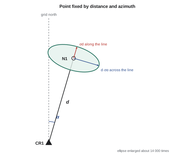
Leah's point N1 is computed from the known pillar CR1 by

The measurements are the distance \(d\) and the azimuth \(\alpha\), which is derived from the direction measured to N1 and the known azimuth of the backsight line. Treating the pillar coordinates and backsight azimuth as error-free for now, the Jacobian is

and, with uncorrelated measurements, the input covariance matrix is

with \(\sigma_\alpha\) in radians. Angular standard deviations must always be converted to radians before they are multiplied by a distance, since one second of arc is \(4.848 \times 10^{-6}\) radians. A useful rule of thumb follows: one second of arc moves a point sideways by about 4.8 mm per kilometre, or 0.5 mm per hundred metres.

The example shows why rules of thumb such as 'the point is good to 6 mm' are incomplete. The point is good to about 2.9 mm along the line and about 6.2 mm across it, and the coordinate standard deviations depend on how the line happens to be oriented relative to grid north. Rotating the same measurement to an azimuth of 90° would swap the roles of easting and northing.

Checking propagation by simulation

A Monte Carlo simulation provides an independent check on any propagation. The idea is to generate thousands of plausible sets of measurements by adding random normal errors with the stated standard deviations to the measured values, compute the result from each set, and then compute the standard deviation of the results directly. If the linearization is valid, the simulated and propagated values agree. Simulation is also the practical tool when a function is too awkward to differentiate, or when measurement errors are not normal.

def T(A): return [list(r) for r in zip(*A)]
def mul(A, B): return [[sum(a * b for a, b in zip(r, c)) for c in zip(*B)] for r in A]
def inv(A):
    n = len(A); M = [list(map(float, r)) + [1.0 if i == j else 0.0 for j in range(n)] for i, r in enumerate(A)]
    for c in range(n):
        p = max(range(c, n), key=lambda r: abs(M[r][c])); M[c], M[p] = M[p], M[c]
        d = M[c][c]; M[c] = [x / d for x in M[c]]
        for r in range(n):
            if r != c:
                f = M[r][c]; M[r] = [x - f * y for x, y in zip(M[r], M[c])]
    return [r[n:] for r in M]
def diag(v): return [[v[i] if i == j else 0.0 for j in range(len(v))] for i in range(len(v))]
def col(v): return [[x] for x in v]

# Propagate distance and azimuth errors into the coordinates of N1
import math, random

E0, N0 = 5000.000, 5000.000
d = 427.200
az = math.radians(16 + 20 / 60)
sd = 0.002 + 2e-6 * d                     # 2 mm + 2 ppm
sa = math.radians(3 / 3600)               # 3 seconds in radians

E = E0 + d * math.sin(az)
N = N0 + d * math.cos(az)
J = [[math.sin(az), d * math.cos(az)],
     [math.cos(az), -d * math.sin(az)]]
Sxx = diag([sd ** 2, sa ** 2])
Syy = mul(mul(J, Sxx), T(J))              # general law: J S J^T

sE, sN, sEN = math.sqrt(Syy[0][0]), math.sqrt(Syy[1][1]), Syy[0][1]
print(f"N1 = {E:.3f} E, {N:.3f} N")
print(f"propagated:  sE = {sE * 1000:.2f} mm, sN = {sN * 1000:.2f} mm, "
      f"cov = {sEN * 1e6:.2f} mm^2, rho = {sEN / (sE * sN):.3f}")
print(f"along the line {sd * 1000:.2f} mm, across the line {d * sa * 1000:.2f} mm")

# Monte Carlo check with a fixed seed so the result is repeatable
random.seed(220)
es, ns = [], []
for _ in range(20000):
    dd = d + random.gauss(0, sd)
    aa = az + random.gauss(0, sa)
    es.append(E0 + dd * math.sin(aa))
    ns.append(N0 + dd * math.cos(aa))
def sdev(v):
    m = sum(v) / len(v)
    return math.sqrt(sum((x - m) ** 2 for x in v) / (len(v) - 1))
print(f"simulated:   sE = {sdev(es) * 1000:.2f} mm, sN = {sdev(ns) * 1000:.2f} mm  (20000 trials)")

N1 = 5120.139 E, 5409.959 N
propagated:  sE = 6.02 mm, sN = 3.25 mm, cov = -8.22 mm^2, rho = -0.421
along the line 2.85 mm, across the line 6.21 mm
simulated:   sE = 6.02 mm, sN = 3.23 mm  (20000 trials)

The propagated and simulated values agree to a few hundredths of a millimetre, which is about as close as twenty thousand random trials can resolve. The small residual difference is sampling noise in the simulation, not a fault in the linearization. If the two disagreed badly, that would be a sign of an error in the Jacobian, a forgotten conversion of seconds to radians, or a function so non-linear that the first-order approximation does not hold.

Trigonometric heighting

The same rules apply in the vertical. A height difference measured by total station is \(\Delta h = S\cos z\), where \(S\) is the slope distance and \(z\) the zenith angle. Its partial derivatives are \(\cos z\) with respect to \(S\) and \(-S\sin z\) with respect to \(z\). For a 312.540 m sight at a zenith angle of 86°30′ with σS = 2.6 mm and σz = 5″, the distance contributes only \(0.061 \times 2.6 = 0.16\) mm, while the zenith angle contributes \(312.5 \times 0.998 \times 2.42 \times 10^{-5} = 7.6\) mm. The height difference of 19.080 m is therefore uncertain by about 7.6 mm, almost entirely because of the zenith angle. That conclusion points directly at how to improve the measurement: measure the zenith angle on both faces several times, and measure reciprocally from both ends to cancel refraction, rather than spending effort on the distance.

Correlated inputs

Field measurements are usually treated as independent, but quantities computed from shared measurements are not, and propagating them as though they were gives the wrong answer. Suppose the coordinates of N1 from the example above are now used to set out a further point. The easting and northing of N1 are correlated, and their full covariance matrix, including the −8.2 mm² term, must be carried forward. Dropping the covariance could understate or overstate the final uncertainty, depending on the geometry. In matrix form there is nothing extra to remember: put the full covariance matrix of all inputs into \(\Sigma_{xx}\), build the Jacobian with respect to all of them, and the law does the rest.

Another common source of correlation is a shared constant. If ten distances are all corrected with the same atmospheric scale factor, and that factor is uncertain, every corrected distance carries the same scale error. The errors are perfectly correlated, and averaging the ten does nothing to reduce that part of the uncertainty. This is the propagation-law view of why systematic errors do not average out.

Using propagation to plan work

Error propagation is most valuable before the field work, when it can still change the plan. If a pier must be set out to 5 mm at 95 per cent from a control point 300 m away, the across-line component alone limits the angle: \(1.96 \times 300\,000 \times \sigma_\alpha \le 5\) mm requires \(\sigma_\alpha \le 8.5 \times 10^{-6}\) rad, or about 1.75″. A 3″ instrument used on one face will not do it from that distance; the choice is between multiple sets of angles, a closer control point or a better instrument. Making that decision in the office costs minutes. Discovering it from a failed check in the field costs a day. Lesson 11 extends this thinking to whole networks.

A budget table is a useful way to present the result. List each error source, its standard deviation, its partial derivative and its contribution, then add the contributions in quadrature. The largest entry is the one worth spending money on, and entries much smaller than the largest can usually be ignored. For Leah's N1, centring errors of 1 mm at the instrument and target would add little compared with the 6.2 mm across-line term, while a 3″ error in the backsight azimuth would be just as important as the measured direction itself.