
GEOM-220 · Lesson 6 of 12 · 22 min
Condition equations
There are two classical ways to set up a least squares adjustment. Lesson 5 used observation equations, which express each observation as a function of unknown parameters such as coordinates. The other way, adjustment by condition equations, uses no parameters at all. Instead it writes down the geometric conditions that the adjusted observations must satisfy: the three angles of a plane triangle must add up to 180°, a closed level loop must have a total height difference of zero, a traverse between two known points must arrive at the known end. The adjustment finds the smallest weighted corrections that make every condition true. The two methods always give identical results when applied to the same problem, but each has situations where it is more natural, and understanding both deepens the understanding of least squares.
How many conditions?
The number of independent conditions equals the redundancy, \(r = n - u\), where \(n\) is the number of observations and \(u\) the number of unknowns that the observations would be needed to determine. For a triangle with three measured angles, two angles are enough to fix its shape, so \(u = 2\) and there is one condition. For a level network of six lines connecting three new benchmarks to two fixed ones, \(u = 3\) and \(r = 3\), so three independent conditions are needed. Finding the right number is easy. Finding a set that is independent, with none expressible as a combination of the others, takes some care: in a level network, the loop conditions around every small loop are independent, but adding a condition around the outer perimeter would duplicate their sum.
This is the main practical drawback of the condition method. In a large network, choosing a complete set of independent conditions by hand is laborious and error-prone, whereas observation equations come one per observation with no thought at all. For this reason commercial network software uses observation equations. The condition method remains attractive for small, self-contained problems such as a single triangle, a closed traverse or a level loop, and it is the natural way to check a network's internal consistency before adjusting it.
The condition model
For linear conditions, write the condition equations on the adjusted observations as
where \(\mathbf{B}\) is an r by n matrix of coefficients, \(\mathbf{c}\) the vector of constants that the conditions must equal, and \(\mathbf{w}\) the vector of misclosures computed from the raw observations. Minimizing \(\mathbf{v}^{\mathsf{T}}\mathbf{P}\mathbf{v}\) subject to these conditions is a constrained minimization, solved by Lagrange multipliers \(\mathbf{k}\) (often called correlates, which is why the method is also known as the method of correlates). The result is
with \(\mathbf{Q} = \mathbf{P}^{-1}\) the cofactor matrix of the observations. The matrix to invert, \(\mathbf{B}\mathbf{Q}\mathbf{B}^{\mathsf{T}}\), is r by r. In observation equations the normal matrix is u by u. When the redundancy is small compared with the number of unknowns, as in a long traverse with only three conditions but dozens of unknown coordinates, the condition method needs a much smaller inversion. That mattered greatly when adjustments were computed by hand, and it explains why older textbooks favour it.
Once the residuals are known, the adjusted observations follow as \(\hat{\boldsymbol{\ell}} = \boldsymbol{\ell} + \mathbf{v}\), and any coordinates or heights can be computed from them along any route, because the adjusted observations are consistent. The a posteriori reference variance is \(\hat{\sigma}_0^2 = \mathbf{v}^{\mathsf{T}}\mathbf{P}\mathbf{v}/r\), exactly as before.
Adjusting the angles of a triangle
The simplest condition adjustment is a plane triangle with all three angles measured. The single condition is \(\alpha + \beta + \gamma = 180^\circ\), so \(\mathbf{B} = \begin{bmatrix} 1 & 1 & 1 \end{bmatrix}\) and \(w\) is the angular misclosure. With equal weights the solution gives each angle a correction of \(-w/3\), the old rule of thumb. With unequal weights, \(\mathbf{B}\mathbf{Q}\mathbf{B}^{\mathsf{T}} = \sigma_1^2 + \sigma_2^2 + \sigma_3^2\) (in units of the reference variance) and each correction is proportional to that angle's variance:
Less precise angles take a larger share of the misclosure, which is exactly what intuition suggests but now in exact proportion.
For a large triangle the condition must use 180° plus the spherical excess, which is the triangle's area divided by the square of the Earth's radius, expressed in seconds. The excess is about 1″ for a triangle of roughly 200 km² and is negligible for engineering triangles a few hundred metres across, but it matters in geodetic networks.
Worked problem
Weighted adjustment of a triangle
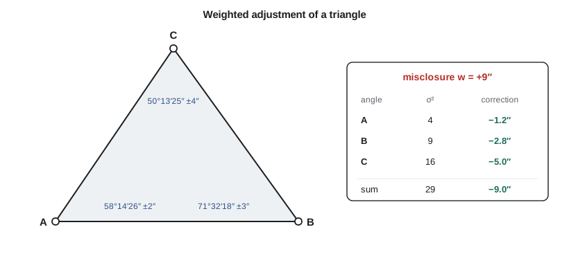
In the bridge network, Leah measures the three angles of a small triangle: A = 58°14′26″ from six sets (σ = 2″), B = 71°32′18″ from three sets (σ = 3″), and C = 50°13′25″ from two sets on a short, steep sight (σ = 4″). Adjust the angles.
Show solution
- \[w = 58^\circ 14' 26'' + 71^\circ 32' 18'' + 50^\circ 13' 25'' - 180^\circ = +9''\]
- \[\sum \sigma_i^2 = 4 + 9 + 16 = 29\ \text{square seconds}\]
- \[v_A = -9 \times \frac{4}{29} = -1.2'', \quad v_B = -9 \times \frac{9}{29} = -2.8'', \quad v_C = -9 \times \frac{16}{29} = -5.0''\]
- \[\hat{A} = 58^\circ 14' 24.8'', \quad \hat{B} = 71^\circ 32' 15.2'', \quad \hat{C} = 50^\circ 13' 20.0''\]
Answer: The adjusted angles sum to exactly 180°. Angle C, the least precise, absorbs more than half of the misclosure, while A, from six sets, changes by little more than a second. An equal split of 3″ each would have pushed the good angle at A further than its precision justifies. With one degree of freedom, \(\hat{\sigma}_0^2 = \sum v_i^2/\sigma_i^2 = 0.39 + 0.87 + 1.54 = 2.79\), so \(\hat{\sigma}_0 = 1.67\), which hints that the angles were somewhat less precise than assumed, though one degree of freedom is far too few to conclude much.
Level loops
Level networks are where the condition method is most intuitive, because every closed loop and every route between two fixed benchmarks gives a condition that anyone who has run a level loop already understands. Consider the network that lesson 7 will adjust by observation equations. Six levelled lines connect three new benchmarks P1, P2 and P3 to two fixed benchmarks, A and B.
The network ties the Coulee Ridge subdivision benchmarks to two geodetic benchmarks published in CGVD2013: A at 902.418 m and B at 915.207 m.
| Line | From | To | Observed rise (m) | Length (km) |
|---|---|---|---|---|
| 1 | A | P1 | 3.4126 | 1.2 |
| 2 | P1 | P2 | 4.1031 | 0.9 |
| 3 | P2 | B | 5.2748 | 1.4 |
| 4 | A | P3 | 6.8392 | 1.6 |
| 5 | P3 | P2 | 0.6773 | 0.8 |
| 6 | P3 | B | 5.9493 | 1.1 |
With six observations and three unknown heights there are three conditions. A convenient independent set is: the loop A to P1 to P2 to P3 and back to A, the loop P3 to P2 to B and back to P3, and the route from A through P3 to B, which must equal the fixed difference B − A = 12.789 m. Writing each as a row of \(\mathbf{B}\), with +1 for a line run in the direction of travel and −1 for one run against it:
The misclosures are all small compared with the 1 mm per √km allowance for loops of three to four kilometres, so there is no sign of a blunder. Weights are the reciprocals of the line lengths, so \(\mathbf{Q}\) is diagonal with the lengths in kilometres.
def T(A): return [list(r) for r in zip(*A)]
def mul(A, B): return [[sum(a * b for a, b in zip(r, c)) for c in zip(*B)] for r in A]
def inv(A):
    n = len(A); M = [list(map(float, r)) + [1.0 if i == j else 0.0 for j in range(n)] for i, r in enumerate(A)]
    for c in range(n):
        p = max(range(c, n), key=lambda r: abs(M[r][c])); M[c], M[p] = M[p], M[c]
        d = M[c][c]; M[c] = [x / d for x in M[c]]
        for r in range(n):
            if r != c:
                f = M[r][c]; M[r] = [x - f * y for x, y in zip(M[r], M[c])]
    return [r[n:] for r in M]
def diag(v): return [[v[i] if i == j else 0.0 for j in range(len(v))] for i in range(len(v))]
def col(v): return [[x] for x in v]

# Condition equation adjustment of the Coulee Ridge level network
import math

lines = [  # (from, to, observed rise in m, length in km)
    ('A', 'P1', 3.4126, 1.2), ('P1', 'P2', 4.1031, 0.9), ('P2', 'B', 5.2748, 1.4),
    ('A', 'P3', 6.8392, 1.6), ('P3', 'P2', 0.6773, 0.8), ('P3', 'B', 5.9493, 1.1)]
HA, HB = 902.418, 915.207
l = [x[2] for x in lines]
Q = diag([x[3] for x in lines])                 # cofactors = lengths in km
B = [[1, 1, 0, -1, -1, 0],                      # loop A-P1-P2-P3-A
     [0, 0, 1, 0, 1, -1],                       # loop P3-P2-B-P3
     [0, 0, 0, 1, 0, 1]]                        # route A-P3-B = HB - HA
c = [0.0, 0.0, HB - HA]
w = [[sum(b * x for b, x in zip(row, l)) - ci] for row, ci in zip(B, c)]
print("misclosures (mm):", ", ".join(f"{x[0] * 1000:+.1f}" for x in w))

k = mul(inv(mul(mul(B, Q), T(B))), w)           # correlates
v = [-x[0] for x in mul(mul(Q, T(B)), k)]       # residuals
adj = [li + vi for li, vi in zip(l, v)]
print("residuals (mm):", ", ".join(f"{x * 1000:+.2f}" for x in v))

check = [sum(b * x for b, x in zip(row, adj)) - ci for row, ci in zip(B, c)]
print("conditions after adjustment (mm):", ", ".join(f"{round(x * 1000, 4) + 0.0:+.4f}" for x in check))

H = {'A': HA}
H['P1'] = H['A'] + adj[0]
H['P2'] = H['P1'] + adj[1]
H['P3'] = H['A'] + adj[3]
print(f"P1 = {H['P1']:.4f}  P2 = {H['P2']:.4f}  P3 = {H['P3']:.4f} m")
print(f"P2 via P3 = {H['P3'] + adj[4]:.4f} m, B via P2 = {H['P2'] + adj[2]:.4f} m (fixed {HB})")
r = len(B)
vtpv = sum(vi ** 2 / x[3] for vi, x in zip(v, lines))
print(f"sigma0 = {math.sqrt(vtpv / r) * 1000:.2f} mm per root km with {r} degrees of freedom")misclosures (mm): -0.8, +2.8, -0.5 residuals (mm): -0.10, -0.07, -1.33, -0.27, -0.70, +0.77 conditions after adjustment (mm): +0.0000, +0.0000, +0.0000 P1 = 905.8305 P2 = 909.9335 P3 = 909.2569 m P2 via P3 = 909.9335 m, B via P2 = 915.2070 m (fixed 915.207) sigma0 = 0.91 mm per root km with 3 degrees of freedom
After adjustment every condition closes to zero, and the heights of P1, P2 and P3 come out the same whichever route is used to compute them: P2 is 909.9335 m whether reached through P1 or through P3. The a posteriori reference standard deviation of 0.91 mm per √km with three degrees of freedom is close to the assumed 1 mm. Lesson 7 adjusts exactly the same data by observation equations, and you will see that the residuals and heights agree to the last digit. That agreement is not a coincidence: both methods minimize the same quantity subject to the same geometry.
Traverses as condition adjustments
A traverse that runs between two known control points, with known azimuths at each end, has three conditions: the angles must carry the starting azimuth to the closing azimuth, and the sums of the easting and northing components must equal the known coordinate differences. The compass rule and transit rule that surveyors learned for distributing traverse misclosures are simplified approximate solutions to this problem. The compass rule, which distributes the linear misclosure in proportion to leg length, corresponds roughly to assuming that the distance and angle errors produce similar position errors along each leg. A rigorous least squares traverse adjustment treats the angles and distances with their proper weights and gives the coordinate precisions as well, which the compass rule cannot do. Most offices now adjust traverses by least squares as part of the wider network, but the compass rule remains a perfectly good check and is still accepted for many small surveys.
The angular condition is linear, but the two coordinate conditions involve sines and cosines of the azimuths, so they must be linearized about the observed values just as observation equations are, and the solution iterated if the misclosures are large. In practice traverse misclosures are small enough that one iteration is usually sufficient.
Comparing the two methods
| Feature | Observation equations | Condition equations |
|---|---|---|
| Equations | One per observation | One per redundant observation |
| Unknowns | Coordinates or heights (u) | None; residuals only |
| Matrix to invert | u × u normal matrix | r × r matrix |
| Setting up | Automatic; easy to program | Must choose independent conditions |
| Adjusted coordinates | Directly, with their covariance | Computed afterwards from adjusted observations |
| Best for | Large networks and software | Small loops, triangles, single traverses, checks |
A third formulation, the general or combined model, mixes both: each equation can contain several observations and several unknowns, as happens when fitting a circle to measured points whose coordinates are all uncertain, or when a GNSS baseline and a levelled height share a geoid model. It reduces to observation equations when each equation has one observation, and to condition equations when there are no unknowns. Photogrammetry and laser scanning often need it; GEOM-310 returns to it for the bundle adjustment.
Common mistakes
MistakeIncluding a dependent condition, such as a perimeter loop that is the sum of smaller loops.
InsteadUse exactly r independent conditions; a dependent set makes BQBᵀ singular.
MistakeSplitting a triangle misclosure equally when the angles have different precisions.
InsteadDistribute in proportion to the variances.
MistakeGetting the sign of a line wrong in a loop.
InsteadUse +1 when the line is run in the direction of travel around the loop and −1 otherwise.
MistakeForgetting spherical excess in a large triangle.
InsteadAdd the excess to 180° when the triangle is large enough for it to matter.
MistakeThinking the two methods give different answers.
InsteadThey give identical results for the same data and weights.
Summary and key terms
- Condition equations constrain the adjusted observations rather than solving for parameters.
- The number of independent conditions equals the redundancy r = n − u.
- The solution is k = (BQBᵀ)⁻¹w and v = −QBᵀk.
- A triangle's misclosure is distributed in proportion to the angle variances.
- Level loops and routes between fixed benchmarks give natural linear conditions.
- The compass rule is an approximation to a condition adjustment of a traverse.
- Observation and condition equations give identical results; software prefers observation equations.
- Condition equation
- An equation that the adjusted observations must satisfy exactly.
- Misclosure
- The amount by which the raw observations fail to satisfy a condition.
- Correlates
- The Lagrange multipliers used to solve a condition adjustment.
- Spherical excess
- The amount by which the angles of a spherical triangle exceed 180°.
- Independent conditions
- A set of conditions none of which can be formed from the others.
- General model
- An adjustment model whose equations each contain several observations and unknowns.
Practice problems
Work each problem on paper first, then reveal the answer to check.
A quadrilateral has all four interior angles measured. How many conditions are there?
Show answer
One angular condition: the four angles must sum to 360°.
Equal-weight triangle angles sum to 179°59′54″. What correction does each receive?
Show answer
+2″ each.
In a level network with 10 lines and 6 new benchmarks tied to one fixed benchmark, how many conditions are needed?
Show answer
r = 10 − 6 = 4.
Triangle angles with σ of 1″, 1″ and 2″ misclose by +6″. Find the corrections.
Show answer
Variances 1, 1, 4 sum to 6: −1″, −1″, −4″.
Why does a closed traverse with fixed ends have three conditions?
Show answer
One angular closure and two coordinate closures (easting and northing).
Lesson quiz · 5 questions
Score 60% or more to complete this lesson.
Create a free account to save your progress, take quizzes and earn a certificate.