
GEOM-220 · Lesson 11 of 12 · 22 min
Network design
Every result in the previous lessons was computed after the field work. Yet the most useful property of least squares for an engineer is that much of it can be computed before anyone leaves the office. The cofactor matrix of the unknowns, \(\mathbf{Q}_{xx} = (\mathbf{A}^{\mathsf{T}}\mathbf{P}\mathbf{A})^{-1}\), depends on the design matrix and the weights, and both of those depend only on where the points are, what will be measured and how precisely. They do not depend on the measured values at all. So error ellipses, redundancy numbers and minimal detectable blunders can all be predicted from a plan of the network and a list of intended observations. This is pre-analysis, and it is the basis of network design: deciding what to measure so that the survey meets its specification at the lowest cost.
Why design matters
A survey that fails its specification after the field work has to be repeated, at the cost of crew time, mobilization and delay to everyone waiting for the control. A survey that greatly exceeds its specification has wasted effort that could have gone elsewhere. Pre-analysis aims between the two. It is required by many agencies for major control projects, and it is good practice for anything where the stakes are high: bridges, tunnels, dams, deformation monitoring, and large GNSS control networks. It also answers practical questions that otherwise rely on guesswork: is it worth occupying this hilltop, do we need angles on every line, will a cheaper instrument do, where should the new pillars go?
The four orders of design
Geodesists classify network design problems into four orders, depending on what is being chosen.
| Order | What is chosen | Typical questions |
|---|---|---|
| Zero | The datum: which points are fixed or how the network is constrained | Hold the pillars, or adjust minimally constrained and transform? |
| First | The configuration: point locations and which observations connect them | Where to place points; which lines to measure |
| Second | The weights: precision of each observation | How many sets; which instrument; GNSS session length |
| Third | Improvement of an existing network | Which extra observations or points strengthen it most? |
In practice, engineers solve the problems together by trial and error: propose a design, compute its precision and reliability, compare with the requirement, adjust, and repeat. A few iterations on a computer usually settle the design. Formal optimization methods exist, but trial and error with good judgement is how most real networks are designed.
Design criteria
Before designing, the requirement must be stated in measurable terms. Precision criteria are the most familiar: the 95 per cent semi-major axis of every point's error ellipse, or of every relative ellipse between specified pairs of points, must be below a stated value. Reliability criteria are equally important: every observation should have a redundancy number above a threshold, often 0.2 to 0.3, and the minimal detectable blunder of every observation, or its effect on the coordinates, should be below a stated value. Cost criteria complete the set: number of set-ups, travel between stations, instrument time and access constraints such as river crossings, traffic or private land.
Precision and reliability are not the same thing. A network can be very precise and poorly reliable if it has just enough observations of very high quality: the ellipses are small, but a blunder in any observation would go undetected and distort the results. A network can also be reliable but imprecise. A well-designed network has both, and adding redundancy usually improves both together.
For the Oldman River bridge, the contractor's specification required that the 95 per cent semi-major axis of every new control point be at most 10 mm relative to the fixed pillars, and Ruth added a reliability requirement of her own: no distance in the network should have an MDB larger than 25 mm, so that a mistake of an inch or so in a prism or instrument height could not slip through.
Pre-analysis of the bridge network
Leah measured the network of lesson 8 from only two set-ups, on the pillars CR1 and CR2. Lesson 10 showed that two of its distances were poorly checked. For the next phase of the project, when two more points will be added on the north approach, Theo asks her to look back at the first network and compare alternative designs, so that the lesson can be applied to the extension.
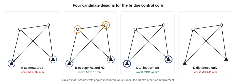
Design A is the network as measured. Design B adds set-ups at N1 and N2, measuring the angles at each new point and reciprocal distances back to the pillars. Design C keeps the two set-ups but uses a 1″ instrument with more sets, giving an angle standard deviation of 1.5″ instead of 3″. Design D omits the angles entirely, as a trilateration-only network. Only the planned coordinates and the standard deviations are needed for the pre-analysis.
def T(A): return [list(r) for r in zip(*A)]
def mul(A, B): return [[sum(a * b for a, b in zip(r, c)) for c in zip(*B)] for r in A]
def inv(A):
    n = len(A); M = [list(map(float, r)) + [1.0 if i == j else 0.0 for j in range(n)] for i, r in enumerate(A)]
    for c in range(n):
        p = max(range(c, n), key=lambda r: abs(M[r][c])); M[c], M[p] = M[p], M[c]
        d = M[c][c]; M[c] = [x / d for x in M[c]]
        for r in range(n):
            if r != c:
                f = M[r][c]; M[r] = [x - f * y for x, y in zip(M[r], M[c])]
    return [r[n:] for r in M]
def diag(v): return [[v[i] if i == j else 0.0 for j in range(len(v))] for i in range(len(v))]
def col(v): return [[x] for x in v]
# Pre-analysis of three designs for the bridge network: no observations needed
import math

X = {'CR1': (5000.0, 5000.0), 'CR2': (5600.0, 5050.0),     # fixed
     'N1': (5120.0, 5410.0), 'N2': (5530.0, 5460.0)}       # planned positions
UNK = ['N1', 'N2']
K95 = 2.4477

def rows(plan):
    A, sig = [], []
    c = lambda p, k: 2 * UNK.index(p) + k if p in UNK else None
    for o in plan:
        row = [0.0] * 4
        if o[0] == 'd':
            a, b, s_ppm = o[1], o[2], o[3]
            dE, dN = X[b][0] - X[a][0], X[b][1] - X[a][1]; d = math.hypot(dE, dN)
            for p, s in ((a, -1), (b, 1)):
                if c(p, 0) is not None:
                    row[c(p, 0)] += s * dE / d; row[c(p, 1)] += s * dN / d
            sig.append(0.002 + s_ppm * 1e-6 * d)
        else:
            at, bs, fs, sec = o[1], o[2], o[3], o[4]
            for p, s in ((fs, 1), (bs, -1)):
                dE, dN = X[p][0] - X[at][0], X[p][1] - X[at][1]; d2 = dE * dE + dN * dN
                for q, s2 in ((p, 1), (at, -1)):
                    if c(q, 0) is not None:
                        row[c(q, 0)] += s * s2 * dN / d2; row[c(q, 1)] -= s * s2 * dE / d2
            sig.append(math.radians(sec / 3600))
        A.append(row)
    return A, sig

def preanalyse(plan):
    A, sig = rows(plan)
    P = diag([1 / s ** 2 for s in sig])
    Q = inv(mul(mul(T(A), P), A))
    worst = 0.0
    for i in (0, 2):
        mid = (Q[i][i] + Q[i + 1][i + 1]) / 2
        a = math.sqrt(mid + math.sqrt(((Q[i][i] - Q[i + 1][i + 1]) / 2) ** 2 + Q[i][i + 1] ** 2))
        worst = max(worst, a)
    AQ = mul(mul(A, Q), T(A))
    red = [1 - AQ[i][i] / sig[i] ** 2 for i in range(len(sig))]
    mdb_d = max(4.13 * s / math.sqrt(r) for o, s, r in zip(plan, sig, red) if o[0] == 'd')
    return K95 * worst * 1000, min(red), mdb_d * 1000, len(plan) - 4

base = [('d', 'CR1', 'N1', 2), ('d', 'CR1', 'N2', 2), ('d', 'CR2', 'N1', 2),
        ('d', 'CR2', 'N2', 2), ('d', 'N1', 'N2', 2),
        ('a', 'CR1', 'CR2', 'N1', 3), ('a', 'CR1', 'N1', 'N2', 3),
        ('a', 'CR2', 'N2', 'CR1', 3), ('a', 'CR2', 'N1', 'N2', 3)]
designs = {
    'A  as measured (2 set-ups)': base,
    'B  add set-ups at N1 and N2': base + [('a', 'N1', 'CR1', 'N2', 3), ('a', 'N1', 'N2', 'CR2', 3),
                                         ('a', 'N2', 'N1', 'CR1', 3), ('a', 'N2', 'CR2', 'N1', 3),
                                         ('d', 'N1', 'CR1', 2), ('d', 'N2', 'CR2', 2)],
    'C  1-second instrument, 2 set-ups': [o if o[0] == 'd' else o[:4] + (1.5,) for o in base],
    'D  distances only (no angles)': base[:5],
}
print(f"{'design':<36}{'r':>3}{'worst 95% axis':>16}{'min r_i':>9}{'worst distance MDB':>20}")
for label, plan in designs.items():
    e95, rmin, mdb, r = preanalyse(plan)
    print(f"{label:<36}{r:>3}{e95:>13.1f} mm{rmin:>9.2f}{mdb:>17.0f} mm")
print("requirement: 95 per cent semi-major axis at most 10 mm, every distance MDB at most 25 mm")design r worst 95% axis min r_i worst distance MDB A as measured (2 set-ups) 5 7.2 mm 0.14 32 mm B add set-ups at N1 and N2 11 6.0 mm 0.41 18 mm C 1-second instrument, 2 set-ups 5 6.2 mm 0.23 24 mm D distances only (no angles) 1 8.3 mm 0.08 41 mm requirement: 95 per cent semi-major axis at most 10 mm, every distance MDB at most 25 mm
All four designs meet the precision requirement, with worst-case 95 per cent semi-axes between 6 and 8.3 mm. Precision alone would suggest the cheapest design is fine. Reliability tells a different story. Design A, as measured, has a minimum redundancy number of 0.14 and a worst distance MDB of 32 mm, failing Ruth's 25 mm requirement. Design D, without angles, is far worse: one degree of freedom, a minimum redundancy number of 0.08 and an MDB of 41 mm. Design C, with the better instrument, just meets the reliability requirement at 24 mm. Design B, with two extra set-ups, meets everything with a wide margin: eleven degrees of freedom, every redundancy number above 0.4, and a worst MDB of 18 mm.
The choice between B and C is now a cost decision with numbers behind it. Design C needs no extra set-ups but requires the firm's best instrument, which is booked on another project, and only just meets the reliability requirement. Design B needs two extra set-ups, about half a day of field time on this site, and leaves margin for an observation or two to be rejected without dropping below the requirement. For the extension of the network, Leah recommends design B's pattern: occupy every new point as well as the pillars.
Worked problem
Effect of adding an observation on precision
In a pre-analysis, a point's variance in one direction is 9.0 mm² from the existing design. A new distance is proposed along exactly that direction with σ = 2.5 mm. Estimate the new variance in that direction, treating the direction as independent of others.
Show solution
- In one dimension, information adds: the inverse variance after adding an observation is the old inverse variance plus the new observation's weight.
- \[\frac{1}{\sigma_{\text{new}}^2} = \frac{1}{9.0} + \frac{1}{2.5^2} = 0.1111 + 0.1600 = 0.2711\]
- \[\sigma_{\text{new}}^2 = 3.69\ \text{mm}^2, \qquad \sigma_{\text{new}} = 1.92\ \text{mm}\]
Answer: The standard deviation in that direction falls from 3.0 mm to about 1.9 mm. The same reasoning, done properly with matrices, is what the pre-analysis program does: each new row added to A adds its own contribution \(\mathbf{a}^{\mathsf{T}}p\,\mathbf{a}\) to the normal matrix. An observation aligned with a point's weakest direction gives the biggest improvement, which is why the best extra observation is usually one that runs along the major axis of the worst ellipse.
Rules of thumb for horizontal networks
Experience with many networks has produced guidelines that pre-analysis usually confirms. Every new point should be connected to at least three others, by observations in at least two clearly different directions. Triangles should be well shaped, with no angle much below 30° or above 120°, because very acute intersections give elongated ellipses. Distances and angles complement each other, controlling along-line and across-line position respectively, so a network should have both. Long sights give better angular precision per point displacement but are more affected by refraction and centring errors on the far target. Occupying new points as well as control points, rather than only shooting to them, adds reliability cheaply. And points that will be used to set out critical structures should be in the strongest part of the network, close to the fixed control.
GNSS network design
The same principles apply to GNSS control networks, such as the 38 km pipeline network that Coulee Geomatics is planning. GNSS baselines measure three coordinate differences each, so a network of independent sessions has more redundancy per baseline than a terrestrial network, but sessions with several receivers produce correlated baselines, and only independent baselines should be counted. Design questions are about the number of receivers, the session lengths, the number of times each point is occupied, and which points are tied to continuously operating reference stations. Common requirements are that every point is occupied at least twice in independent sessions with different satellite geometry, that every new point is connected to at least two control stations or to other new points forming closed loops, and that the network's weakest relative ellipse meets the specification. Pre-analysis uses typical baseline precisions for the session length and the scaling factor found from earlier projects.
For the pipeline, Leah's first design ties the 22 new control points along the right-of-way to two stations of the Canadian Active Control System and to provincial survey control markers at either end, with each point occupied in two sessions on different days. The pre-analysis shows that points in the middle of the route, furthest from control, have the largest ellipses, and that adding a tie to one more control marker near the midpoint reduces their semi-major axes by about a third.
Limits of pre-analysis
Pre-analysis is only as good as its stochastic model. If the assumed standard deviations are optimistic, the predicted ellipses will be too small and the survey may fail when measured. Assumptions should come from the firm's own records of what its instruments and crews actually achieve, ideally from the a posteriori reference variances of past adjustments, rather than from manufacturers' brochures. Pre-analysis also predicts only random error behaviour; systematic errors such as poor grid reductions or refraction near water or hot pavement must be controlled by procedure. Finally, it assumes that the planned observations can actually be made. A site visit to confirm intervisibility, access and safe set-up locations is part of every network design, and a design that relies on sighting across a busy highway or a river in heat shimmer will need revisiting once the crew sees the site.
Common mistakes
MistakeDesigning for precision alone.
InsteadCheck reliability too: redundancy numbers and MDBs.
MistakeUsing manufacturers' specifications in pre-analysis.
InsteadUse standard deviations achieved on past projects.
MistakeCounting all baselines from multi-receiver GNSS sessions.
InsteadCount only independent baselines.
MistakeShooting to new points without occupying them.
InsteadOccupy new points where possible; it adds reliability cheaply.
MistakeSkipping the site visit.
InsteadConfirm intervisibility, access and safety before finalizing the design.
Summary and key terms
- Qxx depends only on A and P, so precision can be predicted before measuring.
- Pre-analysis predicts error ellipses, redundancy numbers and MDBs from the planned design.
- Design orders: zero (datum), first (configuration), second (weights), third (improvement).
- Requirements should cover precision, reliability and cost.
- A design can meet precision requirements and still fail reliability ones.
- The most effective new observation usually runs along the major axis of the worst ellipse.
- Assumed standard deviations should come from the firm's own past results.
- Pre-analysis
- Computing the expected precision and reliability of a planned survey before field work.
- Network design
- Choosing datum, configuration and observation precision to meet requirements at lowest cost.
- Configuration
- The arrangement of points and the observations that connect them.
- Reliability
- A network's ability to detect blunders and limit their effect on results.
- Independent baseline
- A GNSS baseline not derivable from other baselines in the same session.
- Densification
- Adding new points to an existing control network.
Practice problems
Work each problem on paper first, then reveal the answer to check.
Why can pre-analysis be done before any measurements?
Show answer
Qxx = (AᵀPA)⁻¹ depends only on point positions and weights, not on observed values.
A point has variance 16 mm² in its weakest direction. A new distance with σ = 3 mm is added along that direction. What is the new standard deviation?
Show answer
1/σ² = 1/16 + 1/9 = 0.1736, so σ = 2.4 mm.
A four-receiver GNSS session produces how many independent baselines?
Show answer
Three.
Name the design order that chooses how many sets of angles to measure.
Show answer
Second order.
Design X has smaller ellipses but a minimum r_i of 0.05; design Y has slightly larger ellipses and a minimum r_i of 0.35. Which is more reliable?
Show answer
Design Y.
Lesson quiz · 5 questions
Score 60% or more to complete this lesson.
Create a free account to save your progress, take quizzes and earn a certificate.