
GEOM-220 · Lesson 10 of 12 · 23 min
Statistical testing and blunder detection
Least squares will always produce an answer. Feed it observations with a blunder, wrong weights or a disturbed control point and it will still return coordinates, residuals and tidy error ellipses, and nothing in those numbers will announce that something is wrong. The surveyor's protection is statistical testing. Two tests do most of the work. The global test asks whether the residuals as a whole are consistent with the assumed precision of the observations. Data snooping then asks, observation by observation, whether any single residual is too large to be explained by random error. Together with redundancy numbers and minimal detectable blunders, which describe how well each observation is checked, these tools turn an adjustment from a calculation into a quality control process.
The global test
Lesson 3 introduced the a posteriori reference variance \(\hat{\sigma}_0^2 = \mathbf{v}^{\mathsf{T}}\mathbf{P}\mathbf{v}/r\). If the functional model is right, the observations contain no blunders, and the a priori standard deviations are realistic, then \(\mathbf{v}^{\mathsf{T}}\mathbf{P}\mathbf{v}/\sigma_0^2\) follows a chi-square distribution with \(r\) degrees of freedom. Its expected value is \(r\), so \(\hat{\sigma}_0^2/\sigma_0^2\) should be close to one. The global test, also called the chi-square test on the variance factor, checks whether the computed value falls inside the range that chance alone would produce:
With the usual significance level \(\alpha = 5\) per cent, the bounds are the 2.5 and 97.5 per cent points of the chi-square distribution. A value above the upper bound means the residuals are larger than expected: there may be a blunder, the a priori standard deviations may be too optimistic, or the functional model may be missing something, such as a scale error. A value below the lower bound means the residuals are too small: the a priori standard deviations were too pessimistic, which is a less serious fault but still means the reported precisions are wrong. Many software packages test only the upper bound, using a one-tailed test, because large residuals are the main concern.
| Degrees of freedom r | Lower bound (2.5 %) | Upper bound (97.5 %) |
|---|---|---|
| 1 | 0.001 | 5.02 |
| 2 | 0.051 | 7.38 |
| 3 | 0.216 | 9.35 |
| 4 | 0.484 | 11.14 |
| 5 | 0.831 | 12.83 |
| 10 | 3.25 | 20.48 |
| 20 | 9.59 | 34.17 |
| 50 | 32.36 | 71.42 |
For large \(r\), the bounds close in around \(r\): with 50 degrees of freedom the ratio \(\hat{\sigma}_0^2/\sigma_0^2\) must lie between about 0.65 and 1.43. With few degrees of freedom the test is weak, accepting ratios anywhere from 0.17 to 2.6 at \(r = 5\), so a passed global test on a small network is only mild reassurance.
Worked problem
Global test of the bridge network
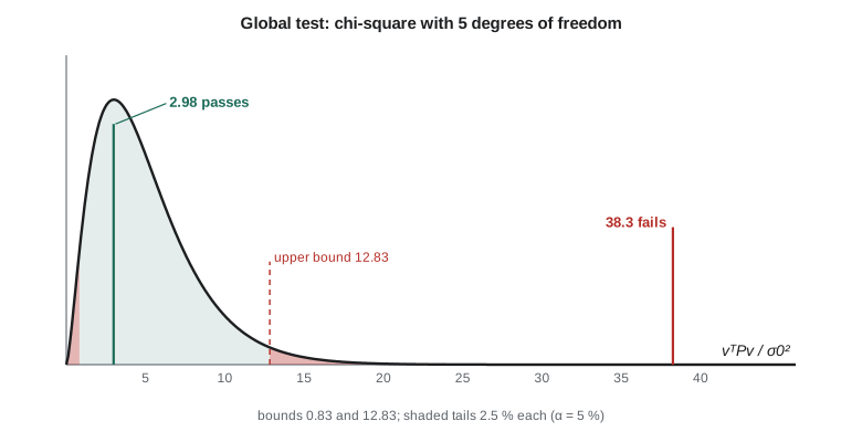
The bridge network of lesson 8 has five degrees of freedom and \(\mathbf{v}^{\mathsf{T}}\mathbf{P}\mathbf{v} = 2.98\) with \(\sigma_0 = 1\). Apply the global test at α = 5 per cent.
Show solution
- \[\chi^2_{5,\,0.025} = 0.831, \qquad \chi^2_{5,\,0.975} = 12.833\]
- \[0.831 < 2.98 < 12.833\]
- \[\hat{\sigma}_0 = \sqrt{2.98/5} = 0.77\]
Answer: The global test passes. The observations fit together as well as their a priori precisions predicted, or slightly better, and there is no evidence of a blunder large enough to disturb the whole adjustment. That does not prove there are no blunders; it says only that any that exist are not large enough, relative to the network's redundancy, to push the overall statistic outside its bounds.
Standardized residuals and data snooping
The global test looks at all residuals together. To find which observation is at fault, each residual must be judged on its own, and that requires its standard deviation. Residuals do not all have the same precision even when the observations do: an observation well checked by the rest of the network can show a large residual, while one that the network can barely check is forced to agree and shows a tiny one. The cofactor matrix of the residuals is
and the standardized residual of observation \(i\) is
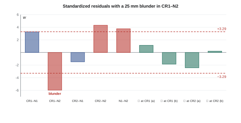
If observation \(i\) contains no blunder, \(w_i\) follows a standard normal distribution. Baarda's data snooping tests each \(w_i\) against a critical value. Because there are many observations and each is tested, a small significance level is used for each test, conventionally \(\alpha_0 = 0.1\) per cent, giving a critical value of 3.29. Any observation with \(|w_i| > 3.29\) is flagged. When \(\sigma_0\) is replaced by the estimate \(\hat{\sigma}_0\) from the same adjustment, the statistic follows Pope's tau distribution instead and the critical value depends on the redundancy, but the procedure is the same.
Data snooping assumes there is at most one blunder at a time. Since a blunder spreads into neighbouring residuals, several standardized residuals may exceed the critical value even when only one observation is bad. The standard procedure is therefore iterative: remove the single observation with the largest \(|w_i|\), readjust, test again, and continue until no residual exceeds the critical value. Removed observations should then be investigated and, wherever possible, remeasured rather than simply discarded.
Redundancy numbers
The diagonal of \(\mathbf{Q}_{vv}\mathbf{P}\) gives the redundancy number \(r_i\) of each observation, a value between 0 and 1. The redundancy numbers sum to the total redundancy \(r\). An observation with \(r_i\) close to 1 is fully checked: a blunder in it shows up almost entirely in its own residual. An observation with \(r_i\) close to 0 is not checked at all: the adjustment simply accepts it, its residual is always near zero, and a blunder in it passes straight into the coordinates. A spur line in a level network has \(r_i = 0\). A useful rule of thumb is that observations with \(r_i\) below about 0.3 are poorly checked, and those below 0.1 are effectively uncontrolled.
Redundancy numbers also explain the size of residuals. A blunder \(\nabla\) in observation \(i\) produces a residual of about \(-r_i\nabla\) in that observation, with the rest spread into its neighbours. If \(r_i = 0.5\), only half of the blunder appears in its own residual.
Minimal detectable blunder
Testing has two kinds of failure. A type I error flags a good observation as a blunder; its probability is \(\alpha_0\). A type II error misses a real blunder; its probability is \(\beta\), and the power of the test is \(1 - \beta\). The minimal detectable blunder (MDB) is the smallest blunder in an observation that data snooping will detect with a chosen power, conventionally 80 per cent:
The MDB is a measure of internal reliability, the network's ability to catch its own mistakes. A distance with \(\sigma = 3\) mm and \(r_i = 0.5\) has an MDB of about 18 mm; with \(r_i = 0.1\) the MDB rises to 39 mm, so a blunder of 30 mm in that distance would probably go unnoticed. The effect of an undetected blunder of MDB size on the adjusted coordinates is called external reliability, and it is what ultimately matters to the user of the coordinates.
Data snooping on the bridge network
To see the tools in action, Theo gives Leah a copy of the bridge network data with a 25 mm blunder deliberately added to the distance CR1–N2, the sort of mistake a wrong prism constant on one set-up might cause, and asks her to find it.
def T(A): return [list(r) for r in zip(*A)]
def mul(A, B): return [[sum(a * b for a, b in zip(r, c)) for c in zip(*B)] for r in A]
def inv(A):
    n = len(A); M = [list(map(float, r)) + [1.0 if i == j else 0.0 for j in range(n)] for i, r in enumerate(A)]
    for c in range(n):
        p = max(range(c, n), key=lambda r: abs(M[r][c])); M[c], M[p] = M[p], M[c]
        d = M[c][c]; M[c] = [x / d for x in M[c]]
        for r in range(n):
            if r != c:
                f = M[r][c]; M[r] = [x - f * y for x, y in zip(M[r], M[c])]
    return [r[n:] for r in M]
def diag(v): return [[v[i] if i == j else 0.0 for j in range(len(v))] for i in range(len(v))]
def col(v): return [[x] for x in v]
# Global test and data snooping on the bridge network with a deliberate 25 mm blunder
import math

fixed = {'CR1': (5000.000, 5000.000), 'CR2': (5600.000, 5050.000)}
start = {'N1': (5121.0, 5408.0), 'N2': (5528.0, 5462.0)}
obs = [  # (kind, at/from, backsight/to, foresight, value in m or (d, m, s))
    ('d', 'CR1', 'N1', None, 427.1997), ('d', 'CR1', 'N2', None, 701.7845 + 0.025),  # blunder
    ('d', 'CR2', 'N1', None, 599.9995), ('d', 'CR2', 'N2', None, 415.9321),
    ('d', 'N1', 'N2', None, 413.0357),
    ('a', 'CR1', 'CR2', 'N1', (291, 4, 38.3)), ('a', 'CR1', 'N1', 'N2', (32, 43, 53.6)),
    ('a', 'CR2', 'N2', 'CR1', (274, 55, 31.8)), ('a', 'CR2', 'N1', 'N2', (43, 26, 31.8))]
RHO = 180 / math.pi * 3600
UNK = ['N1', 'N2']
# Approximate chi-square values for a two-tailed test at alpha = 5 per cent
# (lower 2.5 per cent point, upper 97.5 per cent point), from standard tables
CHI2 = {1: (0.001, 5.024), 2: (0.051, 7.378), 3: (0.216, 9.348),
        4: (0.484, 11.143), 5: (0.831, 12.833), 6: (1.237, 14.449)}
K_SNOOP = 3.29        # Baarda's critical value, alpha0 = 0.1 per cent, normal distribution
DELTA0 = 4.13         # non-centrality for alpha0 = 0.1 per cent and power 80 per cent

def name(o):
    return f"distance {o[1]}-{o[2]}" if o[0] == 'd' else f"angle {o[2]}-{o[1]}-{o[3]}"

def adjust(obs):
    X = dict(fixed); X.update(start)
    c = lambda p, k: 2 * UNK.index(p) + k if p in UNK else None
    for _ in range(10):
        A, w, sig = [], [], []
        for kind, a, b, f, val in obs:
            row = [0.0] * 4
            if kind == 'd':
                dE, dN = X[b][0] - X[a][0], X[b][1] - X[a][1]; d0 = math.hypot(dE, dN)
                for p, s in ((a, -1), (b, 1)):
                    if c(p, 0) is not None:
                        row[c(p, 0)] += s * dE / d0; row[c(p, 1)] += s * dN / d0
                w.append(val - d0); sig.append(0.002 + 2e-6 * val)
            else:
                az = {}
                for p, s in ((f, 1), (b, -1)):
                    dE, dN = X[p][0] - X[a][0], X[p][1] - X[a][1]; d2 = dE * dE + dN * dN
                    az[p] = math.atan2(dE, dN)
                    for q, s2 in ((p, 1), (a, -1)):
                        if c(q, 0) is not None:
                            row[c(q, 0)] += s * s2 * dN / d2; row[c(q, 1)] -= s * s2 * dE / d2
                o = math.radians(val[0] + val[1] / 60 + val[2] / 3600)
                w.append((o - (az[f] - az[b]) + math.pi) % (2 * math.pi) - math.pi)
                sig.append(math.radians(3 / 3600))
            A.append(row)
        P = diag([1 / s ** 2 for s in sig])
        Qxx = inv(mul(mul(T(A), P), A))
        dx = [r[0] for r in mul(Qxx, mul(mul(T(A), P), col(w)))]
        for i, p in enumerate(UNK):
            X[p] = (X[p][0] + dx[2 * i], X[p][1] + dx[2 * i + 1])
        if max(abs(x) for x in dx) < 1e-6:
            break
    v = [-x for x in w]                                  # converged, so v = -w
    AQAt = mul(mul(A, Qxx), T(A))
    qvv = [sig[i] ** 2 - AQAt[i][i] for i in range(len(obs))]
    red = [qvv[i] / sig[i] ** 2 for i in range(len(obs))]  # redundancy numbers
    wst = [v[i] / math.sqrt(qvv[i]) for i in range(len(obs))]
    vtpv = sum(v[i] ** 2 / sig[i] ** 2 for i in range(len(obs)))
    return X, v, red, wst, vtpv, sig

current = list(obs)
for rnd in (1, 2):
    X, v, red, wst, vtpv, sig = adjust(current)
    r = len(current) - 4
    lo, hi = CHI2[r]
    print(f"round {rnd}: r = {r}, vTPv = {vtpv:.2f}, bounds {lo} to {hi} ->",
          "global test passes" if lo < vtpv < hi else "global test FAILS")
    for o, vi, ri, wi in zip(current, v, red, wst):
        unit = f"{vi * 1000:+6.1f} mm" if o[0] == 'd' else f"{vi * RHO:+6.1f} sec"
        flag = "  <- exceeds 3.29" if abs(wi) > K_SNOOP else ""
        print(f"   {name(o):<22} v = {unit}  r_i = {ri:.2f}  w = {wi:+.2f}{flag}")
    worst = max(range(len(current)), key=lambda i: abs(wst[i]))
    if abs(wst[worst]) <= K_SNOOP:
        break
    print(f"   largest |w| is {name(current[worst])}: remove it and readjust")
    current.pop(worst)

print("minimal detectable blunders in the original network (alpha0 0.1 per cent, power 80 per cent):")
X, v, red, wst, vtpv, sig = adjust(obs)
for o, ri, s in zip(obs, red, sig):
    mdb = DELTA0 * s / math.sqrt(ri)
print(f" {name(o):<22} r_i = {ri:.2f} MDB = " + (f"{mdb * 1000:.0f} mm" if o[0] == 'd' else f"{mdb * RHO:.0f} sec"))round 1: r = 5, vTPv = 38.26, bounds 0.831 to 12.833 -> global test FAILS distance CR1-N1 v = +3.6 mm r_i = 0.15 w = +3.28 distance CR1-N2 v = -14.9 mm r_i = 0.54 w = -5.97 <- exceeds 3.29 distance CR2-N1 v = -3.2 mm r_i = 0.45 w = -1.48 distance CR2-N2 v = +4.5 mm r_i = 0.14 w = +4.32 <- exceeds 3.29 distance N1-N2 v = +6.3 mm r_i = 0.36 w = +3.76 <- exceeds 3.29 angle CR2-CR1-N1 v = +3.2 sec r_i = 0.84 w = +1.14 angle N1-CR1-N2 v = -5.2 sec r_i = 0.86 w = -1.85 angle N2-CR2-CR1 v = -6.6 sec r_i = 0.81 w = -2.43 angle N1-CR2-N2 v = +0.6 sec r_i = 0.85 w = +0.21 largest |w| is distance CR1-N2: remove it and readjust round 2: r = 4, vTPv = 2.65, bounds 0.484 to 11.143 -> global test passes distance CR1-N1 v = -0.5 mm r_i = 0.09 w = -0.57 distance CR2-N1 v = +0.6 mm r_i = 0.41 w = +0.28 distance CR2-N2 v = -0.6 mm r_i = 0.04 w = -0.99 distance N1-N2 v = +1.5 mm r_i = 0.27 w = +1.04 angle CR2-CR1-N1 v = +0.5 sec r_i = 0.82 w = +0.17 angle N1-CR1-N2 v = -3.0 sec r_i = 0.84 w = -1.08 angle N2-CR2-CR1 v = -0.7 sec r_i = 0.71 w = -0.28 angle N1-CR2-N2 v = -3.3 sec r_i = 0.80 w = -1.21 minimal detectable blunders in the original network (alpha0 0.1 per cent, power 80 per cent): distance CR1-N1 r_i = 0.15 MDB = 30 mm distance CR1-N2 r_i = 0.54 MDB = 19 mm distance CR2-N1 r_i = 0.45 MDB = 20 mm distance CR2-N2 r_i = 0.14 MDB = 32 mm distance N1-N2 r_i = 0.36 MDB = 20 mm angle CR2-CR1-N1 r_i = 0.84 MDB = 13 sec angle N1-CR1-N2 r_i = 0.86 MDB = 13 sec angle N2-CR2-CR1 r_i = 0.81 MDB = 14 sec angle N1-CR2-N2 r_i = 0.85 MDB = 13 sec
The global test fails decisively: 38.3 against an upper bound of 12.8. Three standardized residuals exceed 3.29, but the largest, −5.97, belongs to the corrupted distance CR1–N2, and removing it and readjusting gives a passing global test with no flagged residuals. Two things in the output are worth studying carefully.
First, the residual of the bad distance is only −14.9 mm, not −25 mm. With a redundancy number of 0.54, about half of the blunder appears in its own residual and the rest is spread over the other observations, which is why CR2–N2 and N1–N2 were also flagged in the first round. Removing them instead would have been wrong, which is why only the single largest standardized residual is removed at each step.
Second, look at the redundancy numbers. The angles have \(r_i\) of about 0.8 to 0.9 and are well checked. The distances CR1–N1 and CR2–N2 have \(r_i\) of only 0.14 to 0.15 and MDBs of about 30 mm, so a blunder of 25 mm in either of them would very probably have gone unnoticed. After CR1–N2 is removed, CR2–N2 drops to \(r_i = 0.04\), almost uncontrolled. The network is adequate for detecting blunders in most observations, but not all, and lesson 11 shows how adding one or two observations would strengthen it.
Beyond data snooping
Data snooping is the most widely taught method, but it has limitations: it assumes one blunder at a time, and with several blunders in poorly checked parts of a network it can remove the wrong observation. Robust estimation methods, such as iteratively reweighted least squares with weights that fall as residuals grow, or minimizing the sum of absolute residuals, can resist several blunders at once. Many professional packages offer a robust option alongside data snooping, and comparing the two is a useful check. Whatever method is used, the best defence is still in the field: independent checks, closed loops, measurements in both directions and careful bookkeeping.
Coulee Geomatics' adjustment report template, which Ruth reviews before sealing any control survey, records the global test result with its degrees of freedom and bounds, every observation removed or reweighted and why, the largest remaining standardized residual, and the observations with redundancy numbers below 0.2. Provincial practice standards expect this kind of documentation for control surveys, and reviewers increasingly ask for it.
Common mistakes
MistakeTreating a passed global test as proof that no blunders exist.
InsteadAlso run data snooping and check redundancy numbers.
MistakeTesting raw residuals against a single limit.
InsteadUse standardized residuals, which account for each residual's own precision.
MistakeRemoving every flagged observation at once.
InsteadRemove only the largest |w|, readjust and test again.
MistakeExpecting a blunder's residual to equal the blunder.
InsteadExpect about r_i times the blunder; the rest spreads to neighbours.
MistakeDiscarding flagged observations without investigation.
InsteadInvestigate and remeasure where possible; record every decision.
Summary and key terms
- The global test compares vᵀPv/σ0² with chi-square bounds for r degrees of freedom.
- A failed global test signals blunders, optimistic weights or a model error.
- Standardized residuals w = v/(σ0√qvv) are tested against 3.29 in data snooping.
- Remove one observation at a time, the largest |w|, and readjust.
- Redundancy numbers between 0 and 1 show how well each observation is checked; they sum to r.
- The minimal detectable blunder is δ0σ/√r_i, with δ0 = 4.13 for the usual settings.
- Robust estimation is an alternative when several blunders may be present.
- Global test
- A chi-square test of whether the overall fit of an adjustment matches the assumed precision.
- Standardized residual
- A residual divided by its own standard deviation.
- Data snooping
- Baarda's procedure for testing standardized residuals one observation at a time.
- Redundancy number
- The share of an observation's blunder that appears in its own residual, between 0 and 1.
- Minimal detectable blunder
- The smallest blunder detectable with a chosen significance and power.
- Internal reliability
- A network's ability to detect blunders in its own observations.
- External reliability
- The effect of an undetected blunder on the adjusted coordinates.
Practice problems
Work each problem on paper first, then reveal the answer to check.
An adjustment has r = 10 and vᵀPv/σ0² = 24.0. Does it pass the two-tailed global test at 5 per cent?
Show answer
No; 24.0 exceeds the upper bound of 20.48.
A residual of −6.0 mm has σv = 1.5 mm. What is its standardized residual, and is it flagged?
Show answer
−4.0; yes, it exceeds 3.29.
Twelve observations have redundancy numbers that sum to 7. How many unknowns does the adjustment have?
Show answer
Five, since the sum equals r = n − u.
Find the MDB for an angle with σ = 2″ and r_i = 0.64.
Show answer
4.13 × 2 / 0.8 = 10.3″.
A blunder of 20 mm occurs in a distance with r_i = 0.25. About how large is its residual?
Show answer
About 5 mm, too small to stand out.
Lesson quiz · 5 questions
Score 60% or more to complete this lesson.
Create a free account to save your progress, take quizzes and earn a certificate.