Wing loading and thrust-to-weight

Two ratios do more than any others to set the size and character of an aircraft: wing loading, the take-off weight divided by wing area, and thrust-to-weight ratio, or for a propeller aircraft its cousin the power loading, installed power divided by weight. Together they decide how fast the aircraft stalls, how short a field it can use, how quickly it climbs, how fast it cruises and how rough its ride is in turbulence. This lesson builds a constraint diagram for the Petrel 19, a plot that shows every performance requirement as a boundary in the plane of wing loading and power loading, and chooses the design point.

Why ratios instead of sizes

Performance equations depend on ratios. Stall speed depends on wing loading and maximum lift coefficient; climb rate depends on excess power per unit weight; take-off distance depends on wing loading divided by thrust or power loading. Working in ratios lets the designer find the right proportions before the take-off mass is final; multiplying by the mass from Lesson 2 then gives wing area and installed power.

Wing loading is quoted here in kilograms per square metre for intuition, so a value of 230 means each square metre of wing carries 230 kg at take-off, or about 2260 N/m². Power loading is quoted in watts of installed shaft power per kilogram of take-off mass. For a hybrid, the installed power that matters for take-off and climb is the rated power of the electric motors that turn the propellers, which does not lapse with altitude or temperature. The turboshaft generators are sized separately for cruise in Lesson 8.

Landing: a ceiling on wing loading

Landing distance depends mainly on the approach speed, which is tied to the stall speed in the landing configuration. For a given maximum lift coefficient, a lower wing loading means a lower stall speed and a shorter landing. Because landing distance does not depend on installed power, the landing requirement appears on the constraint diagram as a vertical line: wing loadings to its right are not allowed.

Arjun calibrates a simple landing model on the Tern's certified performance from the performance course: landing distance from 50 ft on a dry runway of about 0.544 seconds squared per metre times the square of the stall speed, and gravel adding about 38 percent. To land within 1100 m on gravel the dry-runway distance must be under about 797 m, which allows a stall speed of about 38.3 m/s. With a landing maximum lift coefficient of 2.6, the double-slotted flap system proven on the Tern, a hot-day density ratio of 0.95 and a landing mass of 97 percent of take-off mass, the take-off wing loading must not exceed about 233 kg/m².

Take-off: a power boundary that rises with wing loading

Take-off distance grows with wing loading and falls with power loading and take-off lift coefficient. A widely used approach scales the distance with a take-off parameter, wing loading divided by the product of density ratio, take-off lift coefficient and power loading. Arjun again calibrates the constant on the Tern, which needed about 800 m to clear 35 ft at a wing loading of 232 kg/m², 138 W/kg and a take-off lift coefficient of 2.1. For the Petrel the target is 1100 m on gravel, about 957 m on a dry runway after a 15 percent gravel allowance, on a hot day. The required power loading rises in a straight line with wing loading.

Climb with one motor inoperative

A twin must be able to keep climbing after losing one engine on take-off. Requirements set the minimum climb gradient at specific points, with the gear retracted, take-off flaps and the failed engine's propeller in the position it would really be in. For the Petrel the team adopts a design target of a 2 percent gradient at 1.2 times the take-off stall speed with one motor inoperative. Losing one of two motors halves the available power, so the installed power must be at least twice what one motor needs for the climb. This constraint rises slowly with wing loading, because a heavier wing loading means a higher climb speed and more power for the same gradient.

In a series hybrid, losing a motor is not the only failure that matters. Losing a turboshaft generator removes part of the power supply, and the battery must make up the difference for long enough to climb to a safe altitude. Lesson 8 checks this case; here the constraint is the motor-out climb.

Cruise

Cruise at 400 km/h and 3000 m sets a power need that depends on parasite drag, which falls per unit weight as wing loading rises, and induced drag, which rises with wing loading. At low wing loadings the large wing's parasite drag dominates and the required power is high; at higher wing loadings it falls. Because the electric motors do not lapse with altitude, the cruise curve is in the same units as the others; the program assumes cruise at 90 percent of rated motor power and an 80 percent propeller efficiency.

# Constraint analysis for the Petrel 19: required installed motor power per kg against wing loading.
import math
g, rho0 = 9.81, 1.225
sig_hot = 0.95                       # density ratio on a hot day at a sea-level strip
CD0, AR, e = 0.030, 10.0, 0.80
K = 1 / (math.pi * AR * e)
CL_to, CL_land = 2.1, 2.6
eta = 0.75                           # motor-to-thrust efficiency in climb (propeller and installation)
k_to = 999.0                         # take-off constant calibrated on the Tern (AERO-220): s = k (W/S)/(sigma CL P/W)
k_land = 0.544                       # landing distance from 50 ft per (stall speed)^2, dry, s^2/m
gravel_to, gravel_land = 1.15, 1.38
s_field = 1100.0
def takeoff(ws):                     # W/kg needed to clear 35 ft in s_field on gravel
    return k_to * ws / (sig_hot * CL_to * s_field / gravel_to)
def landing_ws_max():                # kg/m2 at MLW = 0.97 MTOW, converted to take-off wing loading
    Vs = math.sqrt(s_field / gravel_land / k_land)
    ws_land = 0.5 * rho0 * sig_hot * Vs ** 2 * CL_land / g
    return ws_land / 0.97, Vs
def climb_oei(ws, G=0.02):           # one motor failed; the other gives the climb gradient G
    Vs = math.sqrt(2 * ws * g / (rho0 * sig_hot * CL_to)); V = 1.2 * Vs
    CL = CL_to / 1.44; CD = 0.050 + K * 1.15 * CL ** 2     # flaps and gear add drag; induced drag up 15 percent
    return 2 * g * V * (CD / CL + G) / eta
def cruise(ws, V=400 / 3.6, sig=0.742):                    # 3000 m, ISA; motors do not lapse with altitude
    q = 0.5 * rho0 * sig * V ** 2
    return V * (q * CD0 / (ws * g) + K * ws * g / q) * g / 0.80 / 0.90   # 0.90: cruise at 90 percent of rated power
ws_land, Vs = landing_ws_max()
print(f"landing limit: stall speed {Vs:.1f} m/s, take-off wing loading at most {ws_land:.0f} kg/m2")
print(" W/S   take-off  OEI climb  cruise   (W/kg of installed motor power)")
for ws in (180, 200, 220, 240, 260):
    print(f"{ws:4d}   {takeoff(ws):6.1f}   {climb_oei(ws):7.1f}   {cruise(ws):6.1f}")
ws = 230
need = max(takeoff(ws), climb_oei(ws), cruise(ws))
print(f"design point W/S {ws} kg/m2: need {need:.1f} W/kg; at 8450 kg that is {need * 8450 / 1e3:.0f} kW in total")

landing limit: stall speed 38.3 m/s, take-off wing loading at most 233 kg/m2
 W/S   take-off  OEI climb  cruise   (W/kg of installed motor power)
 180     94.2     144.4    163.3
 200    104.7     152.2    150.9
 220    115.2     159.7    141.2
 240    125.6     166.8    133.5
 260    136.1     173.6    127.3
design point W/S 230 kg/m2: need 163.2 W/kg; at 8450 kg that is 1379 kW in total

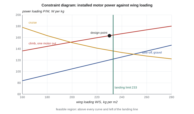
The diagram reads like a map. The feasible region lies above every power curve and to the left of the landing line. The best design point is usually the corner of that region with the least power, because installed power costs mass and money. On the Petrel the corner is set by the landing limit and the one-motor-out climb: at 233 kg/m², the climb requires about 164 W/kg, while take-off on gravel needs only about 122 W/kg and cruise about 136.

Élise chooses a wing loading of 230 kg/m², just inside the landing limit to leave room for growth in landing mass and lift-coefficient uncertainty, and a power loading of 163 W/kg. At 8450 kg this gives a wing area of 36.7 m² and about 1380 kW of installed motor power, two motors of about 700 kW each. The take-off requirement has a comfortable margin, which the operators will appreciate on hot days and soft strips.

Reading what the diagram says

The diagram tells the team what drives the design. Here it is the one-motor-out climb, not take-off or cruise. That points to useful questions. Could a better climb configuration, with lower-drag flap settings or a feathering system that responds faster, reduce the required power? Could the hybrid architecture, which can redistribute power between motors, help? Dr. Nakamura notes that if the surviving motor can be rated for a higher contingency power for a few minutes, the installed rating can be lower, provided motors and inverters are designed and certified for it. These questions go into the trade-study list for Lesson 12.

The diagram also shows what does not matter much. Cruise speed could rise to about 420 km/h without changing the design point, because cruise is not the active constraint. And because take-off is far from active, a slightly smaller flap system might do; Tomasz keeps the Tern's double-slotted flaps anyway because landing, not take-off, sets the wing area.

Wing loading and the ride

Wing loading also affects passengers. An aircraft with low wing loading responds more sharply to gusts, because a given vertical gust changes the lift on a large wing by a larger fraction of the weight. Commuter aircraft with low wing loadings have a reputation for bumpy rides at low altitude. The Petrel's 230 kg/m² is typical of its class: higher than a light trainer's 100 or so, much lower than an airliner's 600. The gust load factors computed in AERO-310 for the Tern carry over roughly, and Marcus will use the Petrel's numbers for its wing loads.

Constraints that were checked and dropped

A full constraint analysis lists more requirements than the four drawn on the Petrel diagram, and part of the work is showing which ones never become active. A service ceiling requirement, a minimum climb rate at the cruise altitude, is easily met by an aircraft that must climb with one motor stopped near the ground. A sustained turn requirement matters for aerobatic and military aircraft but not for a commuter, whose turns are gentle. A minimum climb gradient on the balked landing, with full flaps and gear down, is checked; for the Petrel it lies below the one-motor-out line and drops off the diagram. An approach speed limit, which sets the aircraft's approach category for instrument procedures, is automatically met because the landing line already holds the stall speed down. Arjun writes each of these into the constraint file with its numbers, so a reviewer can see that it was checked rather than forgotten.

Gravel adds its own entries. The take-off distance on gravel is longer than on a paved runway because rolling resistance is higher, a coefficient of about 0.04 to 0.05 on a firm gravel surface compared with about 0.02 on asphalt, and the landing distance is longer because braking friction is lower. Many operators and authorities apply factors to the paved-runway figures for these surfaces. Arjun applies the company's planning factors, which lengthen the take-off distance by about 10 percent and the landing distance by about 15 percent, and the constraint lines in the program already include them. The 1100 m requirement from Lesson 1 is therefore a gravel figure, not a paved one.

Uncertainty and margins

Every line on the diagram rests on estimates: the maximum lift coefficient, the drag polar, the propeller efficiency and the power lapse of the turboshafts with temperature. A good constraint analysis shows how the lines move when those estimates are wrong. The program can be rerun with the maximum lift coefficient 0.2 lower, which moves the landing line left by about 8 percent, or with the parasite drag coefficient 10 percent higher, which raises the climb and cruise lines. The team chooses its design point so that it stays feasible under the pessimistic set of estimates, which is why the point sits a little inside the landing limit rather than on it.

The margin is a deliberate choice, not padding. A wing that is too small cannot be fixed later without a major redesign, while a few percent of extra power can sometimes be found in an engine upgrade. That asymmetry pushes designers toward a slightly larger wing than the diagram's corner suggests. Kenji, who manages the programme budget, asks for the cost of the margin: about 1.5 m² of wing area and roughly 40 kg of structure, which the team judges worth paying.

Constraint analysis for other aircraft types

The same diagram works for any aircraft, but the active lines change. A long-range jet is usually governed by cruise and by the take-off field length at a hot, high airport, and it is drawn with thrust-to-weight instead of power loading. A short-field utility aircraft is governed by landing and take-off. A high-performance glider has almost no power, so its diagram is about wing loading alone. Seeing which line is active for a given mission is one of the first skills a conceptual designer develops, and it is a useful check on any new design: if the active constraints do not match the mission's emphasis, the requirements or the analysis may be wrong.