
STAT-141 · Lesson 9 of 12 · 24 min
Sampling distributions and the central limit theorem
Here is the central problem of statistical inference. We want to know a population parameter, such as the mean commute time of all residents or the proportion of all customers who would use a new service, but we see only one sample. A different random sample would give a somewhat different answer. How much would the answers vary from sample to sample, and what does that tell us about how close our one sample is likely to be to the truth? The answer comes from the idea of a sampling distribution, and its most remarkable fact is the central limit theorem.
Sampling variability
A statistic computed from a random sample is itself a random variable: its value depends on which individuals happened to be chosen. The variation of a statistic from sample to sample is called sampling variability. Sampling variability is not a mistake; it is an unavoidable consequence of looking at part of a population. The goal is to understand it well enough to say how far off our estimate is likely to be.
The sampling distribution of a statistic is the distribution of values it would take over all possible random samples of the same size from the same population. We can never actually take all possible samples, but we can understand sampling distributions in two ways: by simulation, drawing many samples with a computer and watching how the statistic varies, and by mathematics, which gives exact results for the most common statistics.
Simulating a sampling distribution
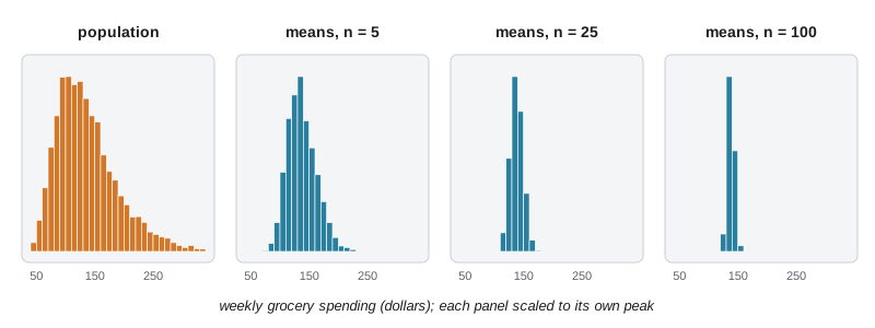
Lucas has a complete record of the weekly grocery spending of all 5,000 households registered with the food bank, which lets him treat them as a population and see what sampling does. The population is skewed to the right, with mean about 140 dollars and standard deviation about 55 dollars. He draws a random sample of 25 households, computes its mean, puts the households back, and repeats the process 2,000 times.
# Simulating the sampling distribution of the sample mean.
import random, statistics as st
random.seed(141)
population = [random.lognormvariate(4.86, 0.38) for _ in range(5000)]   # right-skewed spending, dollars
mu, sigma = st.mean(population), st.pstdev(population)
print(f"population: mean {mu:.1f}, sd {sigma:.1f}, median {st.median(population):.1f} (skewed right)")
for n in (5, 25, 100):
    means = [st.mean(random.sample(population, n)) for _ in range(2000)]
    print(f"n = {n:3d}: mean of sample means {st.mean(means):6.1f}, "
f"sd of sample means {st.stdev(means):5.2f}, sigma/sqrt(n) = {sigma / n ** 0.5:5.2f}")population: mean 138.3, sd 54.6, median 128.1 (skewed right) n = 5: mean of sample means 137.7, sd of sample means 24.27, sigma/sqrt(n) = 24.43 n = 25: mean of sample means 138.2, sd of sample means 10.80, sigma/sqrt(n) = 10.92 n = 100: mean of sample means 138.1, sd of sample means 5.37, sigma/sqrt(n) = 5.46
Three facts stand out in the output. First, the sample means center on the population mean: on average, the sample mean is neither too high nor too low. Second, the sample means vary much less than individual households do, and their spread shrinks as the sample size grows. Third, the spread of the sample means matches the formula \(\sigma/\sqrt{n}\) closely. The histograms, which you can see in the figure, show a fourth fact: even though the population is skewed, the distribution of sample means becomes more symmetric and bell-shaped as n increases.
The mean and standard deviation of the sample mean
Mathematics confirms what the simulation shows. If a simple random sample of size n is drawn from a population with mean \(\mu\) and standard deviation \(\sigma\), the sampling distribution of the sample mean \(\bar{x}\) has mean \(\mu\) and standard deviation \(\sigma/\sqrt{n}\).
Because its mean equals the population mean, we say \(\bar{x}\) is an unbiased estimator of \(\mu\): it does not systematically overshoot or undershoot. The standard deviation \(\sigma/\sqrt{n}\) measures how precise it is, and it shrinks with the square root of the sample size. To halve the variability of the sample mean you need four times as many observations; to cut it to a tenth you need a hundred times as many. This square-root law explains why polls of a few thousand people can be quite precise, and why going from 1,000 to 10,000 respondents improves precision far less than you might expect.
Look at what is missing from the formula: the size of the population. As long as the population is much larger than the sample, at least about ten times larger, the precision of a random sample depends on the sample size, not on what fraction of the population it covers. A random sample of 1,500 voters is about as informative for a country of 40 million as for a country of 340 million. This surprises many people, but it is one of the most useful facts in statistics.
Bias and variability
A good estimator has both low bias and low variability. Think of shooting arrows at a target. Bias means the arrows consistently land off-center; high variability means they scatter widely. A large random sample gives an unbiased, low-variability estimate. A large convenience sample gives a low-variability but biased estimate: all the arrows land close together, but in the wrong place. Increasing sample size reduces variability but does nothing to reduce bias, which must be dealt with through good sampling design, as lesson 2 explained.
| Low variability | High variability | |
|---|---|---|
| Low bias | Large random sample: close to the truth, consistently | Small random sample: right on average, but individual results scatter |
| High bias | Large convenience sample: consistently wrong, with false confidence | Small biased sample: wrong and erratic |
This also explains why we divide by n - 1 when computing a sample variance. Dividing by n would make the sample variance, on average, slightly smaller than the population variance, a small bias. Dividing by n - 1 removes that bias, so the sample variance is an unbiased estimator of the population variance.
The central limit theorem
The simulation showed sample means becoming normal even though the population was skewed. This is not a coincidence. The central limit theorem (CLT) states that when n is large, the sampling distribution of the sample mean is approximately normal, whatever the shape of the population, provided the population has a finite standard deviation. Combined with the formulas above, \(\bar{x}\) is approximately \(N(\mu, \sigma/\sqrt{n})\) for large n.
How large is large? It depends on the population. If the population is itself normal, the sample mean is exactly normal for any sample size. If the population is roughly symmetric, samples of 15 to 20 are usually enough. If it is strongly skewed, like incomes or waiting times, you may need 30, 40 or more. A common rule of thumb is n of at least 30, but it is only a rough guide; very skewed populations or populations with extreme outliers need more.
The central limit theorem is the reason the normal distribution appears everywhere in statistics. Many quantities we care about are averages or totals of many small independent contributions, and the CLT says such quantities tend to be approximately normal. It is also why the methods for confidence intervals and tests in the next lessons work for means even when individual observations are not normal.
# Using the CLT: probability that the mean of 36 waiting times exceeds 15 minutes.
# Individual waits are right-skewed (exponential) with mean 12 and sd 12 minutes.
import random, statistics as st
from statistics import NormalDist
mu, sigma, n = 12, 12, 36
se = sigma / n ** 0.5
print(f"standard deviation of the sample mean: {sigma} / sqrt({n}) = {se:.1f} minutes")
print(f"CLT approximation: P(mean > 15) = {1 - NormalDist(mu, se).cdf(15):.4f}")
random.seed(9)
sims = [st.mean(random.expovariate(1 / mu) for _ in range(n)) for _ in range(20000)]
print(f"simulation:        P(mean > 15) = {sum(m > 15 for m in sims) / len(sims):.4f}")
print(f"P(a single wait > 15) = {sum(random.expovariate(1 / mu) > 15 for _ in range(20000)) / 20000:.3f}")standard deviation of the sample mean: 12 / sqrt(36) = 2.0 minutes CLT approximation: P(mean > 15) = 0.0668 simulation: P(mean > 15) = 0.0719 P(a single wait > 15) = 0.294
The contrast in the output is the heart of the matter. About 29 percent of individual patients wait more than 15 minutes, but the chance that the average wait of 36 patients exceeds 15 minutes is only about 7 percent, because averages are far less variable than individuals. The CLT approximation and the simulation agree reasonably well; the small difference reflects the strong skewness of waiting times, which the approximation smooths over.
The sampling distribution of a sample proportion
Many questions are about proportions rather than means: what fraction of residents would use a new bus route, what fraction of customers redeem a coupon. If a simple random sample of size n is drawn from a large population in which the proportion with some characteristic is p, the sample proportion \(\hat{p}\) (read 'p hat') is the count of successes divided by n. Its sampling distribution has mean p and standard deviation \(\sqrt{p(1-p)/n}\).
So \(\hat{p}\) is an unbiased estimator of p, and its variability shrinks with the square root of the sample size. When both \(np \ge 10\) and \(n(1-p) \ge 10\), the sampling distribution of \(\hat{p}\) is approximately normal. This is the binomial normal approximation from lesson 8 expressed as a proportion instead of a count.
# Sampling distribution of a sample proportion: true p = 0.35, samples of 400.
import random, statistics as st, math
random.seed(35)
p, n = 0.35, 400
phats = [sum(random.random() < p for _ in range(n)) / n for _ in range(5000)]
print(f"mean of sample proportions: {st.mean(phats):.4f} (true p = {p})")
print(f"sd of sample proportions:   {st.stdev(phats):.4f}")
print(f"formula sqrt(p(1-p)/n):     {math.sqrt(p * (1 - p) / n):.4f}")
within = sum(abs(ph - p) <= 2 * math.sqrt(p * (1 - p) / n) for ph in phats) / len(phats)
print(f"share of samples within 2 standard deviations of p: {within:.1%}")mean of sample proportions: 0.3502 (true p = 0.35) sd of sample proportions: 0.0238 formula sqrt(p(1-p)/n): 0.0238 share of samples within 2 standard deviations of p: 95.8%
With 400 respondents and a true proportion of 35 percent, about 95 percent of samples give a sample proportion within about 4.8 percentage points of the truth. Flip that statement around and you have the idea of a margin of error: if we observe a sample proportion, the true proportion is probably within about two standard deviations of it. Lesson 10 makes this precise.
Worked problem
Using the sampling distribution of a mean
Weekly grocery spending by registered households has mean 140 dollars and standard deviation 55 dollars, with a right-skewed distribution. The food bank surveys a random sample of 50 households. What is the probability that the sample mean is more than 155 dollars? Why can we use a normal model even though spending is skewed?
Show solution
- The sampling distribution of the sample mean has mean 140 and standard deviation 55 / sqrt(50) = 7.78 dollars.
- With n = 50 the central limit theorem makes the sample mean approximately normal despite the skewed population.
- Standardize: z = (155 - 140) / 7.78 = 1.93.
- The area to the right of z = 1.93 under the standard normal curve is about 0.027.
- So there is about a 2.7 percent chance that the sample mean exceeds 155 dollars.
Answer: About 0.027; the CLT justifies the normal model for the mean of 50 observations even though individual spending is skewed.
Common mistakes
MistakeConfusing the standard deviation of individuals with the standard deviation of the sample mean.
InsteadThe sample mean varies less: its standard deviation is sigma divided by sqrt(n).
MistakeBelieving a sample must be a large fraction of the population to be accurate.
InsteadFor large populations, precision depends on sample size, not on the sampling fraction.
MistakeThinking the central limit theorem makes individual observations normal.
InsteadIt applies to sample means (and sums), not to the individual values.
MistakeExpecting a larger sample to remove bias.
InsteadLarger samples reduce variability only; bias needs better sampling methods.
MistakeUsing the normal approximation for a proportion with very few expected successes.
InsteadCheck that np and n(1-p) are both at least about 10.
Summary and key terms
- A statistic varies from sample to sample; its sampling distribution describes that variation.
- The sample mean is unbiased for mu and has standard deviation sigma/sqrt(n), which shrinks with the square root of the sample size.
- For large populations, precision depends on the sample size, not the fraction of the population sampled.
- Bias and variability are different: larger samples reduce variability, but only good design removes bias.
- The central limit theorem says the sample mean is approximately normal for large n, whatever the population shape.
- The sample proportion is unbiased for p with standard deviation sqrt(p(1-p)/n), and is approximately normal when np and n(1-p) are at least 10.
- sampling variability
- The variation of a statistic from one random sample to another.
- sampling distribution
- The distribution of a statistic over all possible samples of the same size from the same population.
- unbiased estimator
- A statistic whose sampling distribution has mean equal to the parameter it estimates.
- standard error
- The estimated standard deviation of a statistic's sampling distribution.
- central limit theorem
- The result that the sample mean is approximately normal for large samples, whatever the population shape.
- sample proportion
- The fraction of a sample with a given characteristic, written p hat.
- square-root law
- The fact that the variability of a sample mean or proportion falls in proportion to 1 over the square root of n.
Practice problems
Work each problem on paper first, then reveal the answer to check.
A population has mean 60 and standard deviation 20. Find the mean and standard deviation of the sample mean for n = 100.
Show answer
Mean 60, standard deviation 2.
How large a sample is needed to cut the standard deviation of the sample mean in half compared with n = 50?
Show answer
n = 200.
A survey of 1,000 adults is used in both Canada and the United States. Which is more precise?
Show answer
About the same: precision depends on sample size, not population size.
Does the central limit theorem say that a large sample of incomes will be normally distributed?
Show answer
No; it says the sample mean is approximately normal, not the individual incomes.
For p = 0.2 and n = 400, find the standard deviation of the sample proportion.
Show answer
sqrt(0.2 x 0.8 / 400) = 0.02.
Can the normal approximation be used for p hat with p = 0.02 and n = 100?
Show answer
No: np = 2 is less than 10.
A huge online opt-in survey gives very consistent results every week. Does that mean it is accurate?
Show answer
Not necessarily: low variability does not rule out bias.
Why do we divide by n - 1 in the sample variance?
Show answer
To make the sample variance an unbiased estimator of the population variance.
Lesson quiz · 5 questions
Score 60% or more to complete this lesson.
Create a free account to save your progress, take quizzes and earn a certificate.