Random variables and the binomial distribution

Probability becomes much more useful when outcomes are numbers. The number of customers who redeem a coupon, the number of patients who miss an appointment, the payout on an insurance policy and the winnings from a lottery ticket all take numerical values by chance. This lesson introduces random variables and their probability distributions, the mean or expected value and the standard deviation of a random variable, and the binomial distribution, the most widely used model for counts of successes.

Random variables

A random variable is a numerical outcome of a random phenomenon. We usually name random variables with capital letters such as X or Y. A discrete random variable takes a list of separate values, often counts: the number of heads in four coin tosses, the number of café visits a customer makes in a week, the number of defective items in a batch. A continuous random variable takes any value in an interval, such as a waiting time or a weight; the normal distribution of lesson 5 is the most important continuous model.

The probability distribution of a discrete random variable lists its possible values and their probabilities. The probabilities must each be between 0 and 1 and must add to 1. Owen studies the weekly visits of loyalty app members and models the number of visits X in a randomly chosen week as follows.

From the distribution we can answer questions directly. The probability that a member visits at least three times is P(X ≥ 3) = 0.15 + 0.10 + 0.05 = 0.30. The probability of at least one visit is 1 - P(X = 0) = 0.80, using the complement rule.

Expected value

The mean of a random variable, also called its expected value, is the long-run average value it would take over many repetitions. For a discrete random variable it is a weighted average of the possible values, each weighted by its probability: \(\mu_X = E(X) = \sum x_i\,p_i\). For weekly visits, \(\mu = 0(0.20) + 1(0.25) + 2(0.25) + 3(0.15) + 4(0.10) + 5(0.05) = 1.85\) visits. No member makes 1.85 visits in any particular week; the expected value describes the average over many weeks or many members.

The variance of a random variable is the weighted average of squared deviations from the mean, \(\sigma^2_X = \sum (x_i - \mu)^2 p_i\), and the standard deviation \(\sigma_X\) is its square root. They measure how much the random variable varies around its mean, just as the sample variance and standard deviation do for data.

# Mean and standard deviation of a discrete random variable (weekly visits).
import math
values = [0, 1, 2, 3, 4, 5]
probs = [0.20, 0.25, 0.25, 0.15, 0.10, 0.05]
assert abs(sum(probs) - 1) < 1e-12
mu = sum(x * p for x, p in zip(values, probs))
var = sum((x - mu) ** 2 * p for x, p in zip(values, probs))
print(f"expected visits per week: {mu:.2f}")
print(f"variance: {var:.4f}, standard deviation: {math.sqrt(var):.3f}")
print(f"P(at least 3 visits) = {sum(p for x, p in zip(values, probs) if x >= 3):.2f}")
# Expected weekly visits from 1,000 members
print(f"expected visits from 1,000 members: {1000 * mu:.0f}")

expected visits per week: 1.85
variance: 2.0275, standard deviation: 1.424
P(at least 3 visits) = 0.30
expected visits from 1,000 members: 1850

Expected values are how businesses and governments plan under uncertainty. The café can expect about 1,850 visits per week from 1,000 members, even though no one can say what any individual member will do. Means also behave simply when random variables are combined: the mean of a sum is the sum of the means, and multiplying a random variable by a constant multiplies its mean by the same constant. Variances add too, but only when the random variables are independent.

Expected value in insurance and gambling

Insurance companies stay in business because of expected values. Suppose 1 in 500 policyholders makes a claim of 20,000 dollars in a year and the rest claim nothing. The expected claim per policy is \(20000 \times \frac{1}{500} = 40\) dollars. If the company charges a premium of 60 dollars, it expects to earn 20 dollars per policy on average to cover costs and profit. Any one policyholder either pays 60 and gets nothing back, or gets 20,000; but across hundreds of thousands of policies the law of large numbers makes the company's average outcome very predictable. Policyholders accept a negative expected value because they want protection against a large loss they could not afford.

Games of chance work the same way, from the other side. A casino game or lottery is designed so that the player's expected winnings per bet are less than the price of the bet.

U.S. state lotteries return roughly half of ticket sales as prizes on average and use the rest for state programs, administration and retailer commissions. For a ticket in a game like Powerball, the expected value of prizes is therefore well under the ticket price: on average a player gets back only around half of what they spend. Very large jackpots raise the expected value of the top prize, but they also attract more players, which raises the chance that the jackpot will be shared, and advertised jackpots are usually annuity values before taxes.

# Expected value of a simple raffle: 2,000 tickets sold at 10 dollars each.
prizes = {5000: 1, 500: 4, 50: 20}          # prize amount: number of such prizes
tickets = 2000
price = 10
ev_prize = sum(amount * count for amount, count in prizes.items()) / tickets
print(f"expected prize per ticket: {ev_prize:.2f} dollars")
print(f"expected net gain per ticket: {ev_prize - price:+.2f} dollars")
print(f"share of sales returned as prizes: {ev_prize / price:.0%}")

expected prize per ticket: 4.00 dollars
expected net gain per ticket: -6.00 dollars
share of sales returned as prizes: 40%

The binomial setting

Many counts arise from a simple situation. A fixed number n of trials (observations) is made. Each trial has two possible outcomes, called success and failure. The trials are independent. The probability of success, p, is the same on every trial. This is the binomial setting, and the count X of successes in the n trials has the binomial distribution with parameters n and p, written B(n, p).

Examples abound. The café mails a coupon to 20 customers, each of whom redeems it with probability 0.15, independently: the number of redemptions is B(20, 0.15). The clinic books 40 appointments, each missed with probability 0.08: the number missed is B(40, 0.08). A quality inspector checks 50 items from a production line that makes 2 percent defectives: the number of defectives is B(50, 0.02). In each case check the four conditions; if the trials influence each other or the probability changes from trial to trial, the binomial model may not fit.

Sampling from a population is not exactly independent, because once you have chosen one person the population has changed slightly. As long as the sample is less than about 10 percent of the population, the difference is negligible and the binomial model works well. This is why counts in random samples, such as the number of poll respondents who support a policy, are treated as binomial.

Binomial probabilities

The probability of exactly k successes in n binomial trials is \(P(X = k) = \binom{n}{k} p^k (1 - p)^{n - k}\). The factor \(p^k(1-p)^{n-k}\) is the probability of any one particular arrangement of k successes and n - k failures, and \(\binom{n}{k}\) counts how many such arrangements there are. The mean and standard deviation of a binomial random variable have simple formulas: \(\mu = np\) and \(\sigma = \sqrt{np(1 - p)}\).

# Binomial probabilities: coupon mailed to 20 customers, each redeems with probability 0.15.
from math import comb, sqrt
n, p = 20, 0.15
pmf = [comb(n, k) * p ** k * (1 - p) ** (n - k) for k in range(n + 1)]
for k in range(8):
    print(f"P(X = {k}) = {pmf[k]:.4f}  " + "#" * round(100 * pmf[k]))
print(f"P(X >= 5) = {sum(pmf[5:]):.4f}")
print(f"mean = np = {n * p:.1f}, standard deviation = sqrt(np(1-p)) = {sqrt(n * p * (1 - p)):.3f}")

P(X = 0) = 0.0388  ####
P(X = 1) = 0.1368  ##############
P(X = 2) = 0.2293  #######################
P(X = 3) = 0.2428  ########################
P(X = 4) = 0.1821  ##################
P(X = 5) = 0.1028  ##########
P(X = 6) = 0.0454  #####
P(X = 7) = 0.0160  ##
P(X >= 5) = 0.1702
mean = np = 3.0, standard deviation = sqrt(np(1-p)) = 1.597

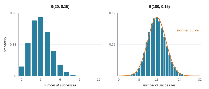
Spreadsheets and statistical software compute binomial probabilities directly; in a spreadsheet the function is usually BINOM.DIST. In practice you rarely need the formula by hand, but understanding it helps you see when the binomial model applies and when it does not.

Overbooking: a binomial application

Airlines, hotels and clinics overbook because some customers do not show up. The clinic has 30 appointment slots each afternoon, and historically each booked patient misses an appointment with probability 0.10, independently. If it books 32 patients, how often will more than 30 show up? The number who show up is B(32, 0.90), and the probability that more than 30 arrive is P(X = 31) + P(X = 32).

# Overbooking: book 32 patients for 30 slots when each shows up with probability 0.9.
from math import comb
def show_prob(n, p, k):
    return comb(n, k) * p ** k * (1 - p) ** (n - k)
p_show = 0.90
for booked in (30, 31, 32, 33, 34):
    over = sum(show_prob(booked, p_show, k) for k in range(31, booked + 1))
    expected = booked * p_show
    print(f"booked {booked}: expected arrivals {expected:4.1f}, P(more than 30 arrive) = {over:.3f}")

booked 30: expected arrivals 27.0, P(more than 30 arrive) = 0.000
booked 31: expected arrivals 27.9, P(more than 30 arrive) = 0.038
booked 32: expected arrivals 28.8, P(more than 30 arrive) = 0.156
booked 33: expected arrivals 29.7, P(more than 30 arrive) = 0.346
booked 34: expected arrivals 30.6, P(more than 30 arrive) = 0.554

The output lets the clinic choose a policy. Booking 32 patients, the clinic expects about 29 arrivals and has roughly a 15 percent chance of more than 30 patients arriving. Whether that risk is acceptable depends on the cost of an empty slot compared with the cost of an overcrowded afternoon, which is a management decision, not a statistical one. The statistics make the trade-off explicit.

The normal approximation to the binomial

When n is large, binomial probabilities become tedious to add up, and the binomial distribution looks more and more like a normal curve. A common rule of thumb says the normal approximation is adequate when both \(np \ge 10\) and \(n(1 - p) \ge 10\). Then X is approximately \(N(np, \sqrt{np(1-p)})\).

For example, if 15 percent of 1,000 mailed coupons are redeemed on average, the number redeemed is B(1000, 0.15), with mean 150 and standard deviation \(\sqrt{1000 \times 0.15 \times 0.85} = 11.3\). The probability that 175 or more are redeemed is approximately the area above \((175 - 150)/11.3 = 2.21\) under the standard normal curve, about 0.013. The exact binomial probability, computed below, is about 0.016, so the approximation is in the right range but a little low.

# Normal approximation to B(1000, 0.15): P(X >= 175), exact vs approximate.
from math import comb, sqrt
from statistics import NormalDist
n, p = 1000, 0.15
exact = sum(comb(n, k) * p ** k * (1 - p) ** (n - k) for k in range(175, n + 1))
mu, sd = n * p, sqrt(n * p * (1 - p))
approx = 1 - NormalDist(mu, sd).cdf(175)
approx_cc = 1 - NormalDist(mu, sd).cdf(174.5)     # with a continuity correction
print(f"mean {mu:.0f}, sd {sd:.2f}")
print(f"exact binomial P(X >= 175)      = {exact:.4f}")
print(f"normal approximation            = {approx:.4f}")
print(f"normal with continuity correction = {approx_cc:.4f}")

mean 150, sd 11.29
exact binomial P(X >= 175)      = 0.0164
normal approximation            = 0.0134
normal with continuity correction = 0.0150

The approximation improves if we use 174.5 instead of 175, a small adjustment called the continuity correction, which accounts for the fact that the binomial count jumps in whole numbers while the normal curve is continuous. The same normal approximation underlies the confidence intervals and tests for proportions in lessons 10 and 11.