
STAT-141 · Lesson 12 of 12 · 28 min
Capstone: comparing groups, chi-square tests and using statistics responsibly
Most real questions compare groups. Did customers who received the invitation visit more often than those who did not? Do younger and older residents get to work differently? Did patients' blood pressure fall after a lifestyle program? This final lesson extends the confidence intervals and tests of lessons 10 and 11 to comparisons of two proportions, two means and paired measurements; introduces the chi-square tests for categorical data; and then steps back to ask how to use statistics responsibly, from reading research to running business experiments. It closes the Community Data Lab's year by working through its main projects from question to conclusion.
Comparing two proportions
Back in lesson 2, the café randomly assigned 600 loyalty members to receive an invitation to a new rewards tier (300 members) or not (300 members). After two months, 96 of the invited members and 66 of the others had made at least eight visits. The sample proportions are 0.32 and 0.22. Is the difference of 10 percentage points larger than chance would produce?
For two independent samples, the difference in sample proportions \(\hat{p}_1 - \hat{p}_2\) estimates the difference in population proportions \(p_1 - p_2\). For a confidence interval, its standard error is \(\sqrt{\frac{\hat{p}_1(1-\hat{p}_1)}{n_1} + \frac{\hat{p}_2(1-\hat{p}_2)}{n_2}}\). For a test of \(H_0: p_1 = p_2\), we use a pooled proportion \(\hat{p}\), the overall proportion of successes in both samples combined, because under the null hypothesis the two groups share one proportion: \(z = \frac{\hat{p}_1 - \hat{p}_2}{\sqrt{\hat{p}(1-\hat{p})(1/n_1 + 1/n_2)}}\). The conditions are independent random samples or random assignment, and at least about 10 successes and 10 failures in each group.
# Two-proportion z test and confidence interval: invited vs not invited.
import math
from statistics import NormalDist
x1, n1 = 96, 300      # invited: members with 8 or more visits
x2, n2 = 66, 300      # control
p1, p2 = x1 / n1, x2 / n2
pool = (x1 + x2) / (n1 + n2)
z = (p1 - p2) / math.sqrt(pool * (1 - pool) * (1 / n1 + 1 / n2))
p_two = 2 * (1 - NormalDist().cdf(abs(z)))
se = math.sqrt(p1 * (1 - p1) / n1 + p2 * (1 - p2) / n2)
print(f"p1 = {p1:.3f}, p2 = {p2:.3f}, difference = {p1 - p2:.3f}")
print(f"pooled proportion = {pool:.3f}, z = {z:.2f}, two-sided p-value = {p_two:.4f}")
print(f"95% CI for p1 - p2: ({p1 - p2 - 1.96 * se:.3f}, {p1 - p2 + 1.96 * se:.3f})")p1 = 0.320, p2 = 0.220, difference = 0.100 pooled proportion = 0.270, z = 2.76, two-sided p-value = 0.0058 95% CI for p1 - p2: (0.029, 0.171)
The p-value is well below 0.05, so the difference is unlikely to be chance, and because the invitation was randomly assigned, the café can reasonably conclude that the invitation caused the increase. The confidence interval says the improvement in the proportion of frequent visitors is probably somewhere between about 3 and 17 percentage points, a wide range that the café should weigh against the cost of the program before rolling it out.
Comparing two means
To compare the means of a quantitative variable in two independent groups, such as the average number of visits by invited and control members, use the two-sample t procedures. The estimate is \(\bar{x}_1 - \bar{x}_2\), with standard error \(\sqrt{s_1^2/n_1 + s_2^2/n_2}\), and the test statistic for \(H_0: \mu_1 = \mu_2\) is \(t = \frac{\bar{x}_1 - \bar{x}_2}{\sqrt{s_1^2/n_1 + s_2^2/n_2}}\). Software computes appropriate degrees of freedom with a formula known as Welch's approximation; this version does not assume the two groups have equal standard deviations and is the recommended default.
# Two-sample (Welch) t test: visits over two months, invited vs control (invented data).
import random, statistics as st
from scipy import stats
random.seed(141)
invited = [max(0, round(random.gauss(7.4, 3.6))) for _ in range(300)]
control = [max(0, round(random.gauss(6.5, 3.4))) for _ in range(300)]
res = stats.ttest_ind(invited, control, equal_var=False)
diff = st.mean(invited) - st.mean(control)
se = (st.variance(invited) / 300 + st.variance(control) / 300) ** 0.5
print(f"mean visits: invited {st.mean(invited):.2f}, control {st.mean(control):.2f}, difference {diff:.2f}")
print(f"Welch t = {res.statistic:.2f}, two-sided p-value = {res.pvalue:.4f}")
print(f"approximate 95% CI for the difference: ({diff - 1.96 * se:.2f}, {diff + 1.96 * se:.2f}) visits")mean visits: invited 7.38, control 6.66, difference 0.73 Welch t = 2.62, two-sided p-value = 0.0090 approximate 95% CI for the difference: (0.18, 1.27) visits
Invited members made about three-quarters of a visit more over two months, on average, and the interval, roughly 0.2 to 1.3 visits, excludes zero. At an average purchase of a few dollars, that difference is easy to translate into revenue, which is exactly the kind of practical judgment a significance test cannot make for you.
Paired data
Sometimes the two sets of measurements are not independent but come in pairs: the same people measured before and after a program, twins, or the same stores in two months. Analyzing paired data as two independent samples throws away valuable information. Instead, compute the difference for each pair and apply the one-sample t procedures of lessons 10 and 11 to the differences.
The clinic ran an eight-week walking and nutrition program for 20 adults with elevated blood pressure and measured each person's systolic pressure before and after.
# Paired t test: systolic blood pressure before and after an 8-week program (invented, mmHg).
import statistics as st
from scipy import stats
before = [148, 152, 139, 160, 145, 150, 142, 158, 147, 155, 141, 149, 153, 146, 162, 144, 151, 157, 143, 150]
after  = [141, 147, 138, 151, 142, 141, 140, 150, 144, 149, 139, 147, 145, 145, 152, 139, 148, 149, 142, 143]
d = [b - a for b, a in zip(before, after)]
print("differences (before - after):", d)
print(f"mean difference = {st.mean(d):.2f} mmHg, sd = {st.stdev(d):.2f}")
paired = stats.ttest_rel(before, after)
print(f"paired t = {paired.statistic:.2f}, two-sided p-value = {paired.pvalue:.6f}")
wrong = stats.ttest_ind(before, after, equal_var=False)
print(f"(analysed wrongly as independent samples: p-value = {wrong.pvalue:.4f})")differences (before - after): [7, 5, 1, 9, 3, 9, 2, 8, 3, 6, 2, 2, 8, 1, 10, 5, 3, 8, 1, 7] mean difference = 5.00 mmHg, sd = 3.08 paired t = 7.26, two-sided p-value = 0.000001 (analyzed wrongly as independent samples: p-value = 0.0071)
Pressure fell by about 5 mmHg on average, and the paired test gives very strong evidence of a change. Analyzed wrongly as two independent groups, the same data look far less convincing: the p-value is thousands of times larger, because the large differences between people swamp the consistent within-person drop. With a smaller or noisier study, that mistake could hide a real effect entirely. One important caution: this study had no control group, so the drop could also reflect regression to the mean (people enrol when their readings are unusually high), seasonal changes or simply getting used to the measurement. A randomized comparison with a control group would be needed to credit the program itself.
Chi-square tests for categorical data
When both variables are categorical, comparisons are made with chi-square tests. The chi-square statistic compares the observed counts in each cell of a table with the counts you would expect if the null hypothesis were true: \(\chi^2 = \sum \frac{(\text{observed} - \text{expected})^2}{\text{expected}}\). Large values mean the observed counts are far from what the null hypothesis predicts. The p-value comes from a chi-square distribution, a right-skewed family of distributions identified by degrees of freedom.
A goodness-of-fit test asks whether the counts for one categorical variable match a hypothesized set of proportions. For example, the food bank expects visits to be spread evenly over its five weekday opening days; it counts visits over a month to see whether demand is really even. The expected count for each day is the total divided by five, and the degrees of freedom are the number of categories minus one.
# Chi-square goodness of fit: are food bank visits spread evenly over five weekdays?
from scipy import stats
observed = {"Mon": 212, "Tue": 168, "Wed": 175, "Thu": 181, "Fri": 234}
total = sum(observed.values())
expected = [total / 5] * 5
chi2, p = stats.chisquare(list(observed.values()), f_exp=expected)
for (day, o), e in zip(observed.items(), expected):
    print(f"{day}: observed {o}, expected {e:.0f}, contribution {(o - e) ** 2 / e:.2f}")
print(f"chi-square = {chi2:.2f} with {len(observed) - 1} df, p-value = {p:.5f}")Mon: observed 212, expected 194, contribution 1.67 Tue: observed 168, expected 194, contribution 3.48 Wed: observed 175, expected 194, contribution 1.86 Thu: observed 181, expected 194, contribution 0.87 Fri: observed 234, expected 194, contribution 8.25 chi-square = 16.13 with 4 df, p-value = 0.00284
A test of independence asks whether two categorical variables measured on the same individuals are related. Lucas's transit survey cross-classifies 400 residents by age group and usual travel mode. Under the null hypothesis that travel mode is independent of age group, the expected count in each cell is (row total x column total) / grand total. The degrees of freedom are (number of rows - 1) x (number of columns - 1). Both chi-square tests require random sampling and expected counts of at least about 5 in every cell.
# Chi-square test of independence: travel mode by age group (invented survey of 400).
from scipy import stats
modes = ["car", "bus", "walk or bike"]
table = [[ 88, 38, 34],     # under 30
         [164, 26, 50]]     # 30 and over
chi2, p, df, expected = stats.chi2_contingency(table)
for label, row, erow in zip(["under 30", "30 and over"], table, expected):
    print(f"{label:<12}" + "  ".join(f"{m}: {o} (exp {e:.1f})" for m, o, e in zip(modes, row, erow)))
print(f"chi-square = {chi2:.2f}, df = {df}, p-value = {p:.5f}")
for label, row in zip(["under 30", "30 and over"], table):
print(f"{label}: " + ", ".join(f"{m} {o / sum(row):.0%}" for m, o in zip(modes, row)))under 30 car: 88 (exp 100.8) bus: 38 (exp 25.6) walk or bike: 34 (exp 33.6) 30 and over car: 164 (exp 151.2) bus: 26 (exp 38.4) walk or bike: 50 (exp 50.4) chi-square = 12.73, df = 2, p-value = 0.00172 under 30: car 55%, bus 24%, walk or bike 21% 30 and over: car 68%, bus 11%, walk or bike 21%
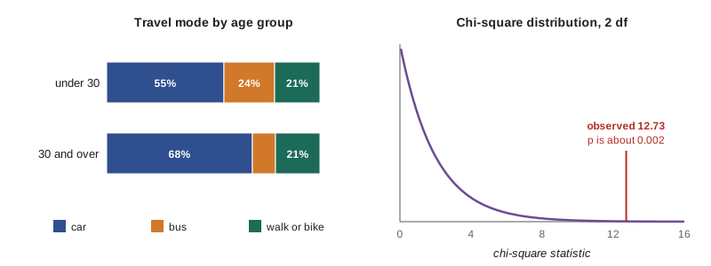
The test shows strong evidence that travel mode is related to age group, and the row percentages show how: younger residents take the bus at roughly twice the rate of older residents, who drive more. Because this is an observational survey, the association does not tell us why; income, car ownership, student fare discounts and where people live are all plausible explanations.
Beyond two groups, and beyond normality
To compare means across three or more groups, such as average spending at four store locations, analysis of variance (ANOVA) tests whether all the group means are equal by comparing the variation between groups with the variation within groups. If the test is significant, follow-up comparisons identify which groups differ, with adjustments for making several comparisons. STAT-151 and later courses develop ANOVA in detail.
When samples are small and the data are strongly skewed or have outliers, the t procedures may not be reliable. Nonparametric tests, such as the Wilcoxon rank-sum test (also called the Mann–Whitney test) for two independent groups and the Wilcoxon signed-rank test for paired data, work with the ranks of the observations rather than their values, so they are resistant to outliers and do not assume normality. They answer slightly different questions, roughly about medians or typical values rather than means, and are a good companion check when the conditions for t are doubtful.
| Question | Data | Procedure |
|---|---|---|
| Is a proportion different from a claimed value? | One categorical variable (two outcomes) | One-proportion z test and interval |
| Is a mean different from a claimed value? | One quantitative variable | One-sample t test and interval |
| Do two groups differ in a proportion? | Two independent samples, two outcomes | Two-proportion z test and interval |
| Do two groups differ in a mean? | Two independent samples, quantitative | Two-sample (Welch) t test and interval |
| Did measurements change within individuals? | Paired quantitative data | Paired t on the differences (or signed-rank) |
| Do counts match expected proportions? | One categorical variable, several categories | Chi-square goodness of fit |
| Are two categorical variables related? | Two-way table of counts | Chi-square test of independence |
| Do three or more group means differ? | Several independent samples, quantitative | One-way ANOVA |
| Are two quantitative variables linearly related? | Paired quantitative variables | Correlation and regression (lesson 6) |
A/B testing in business
The café's invitation study is an example of an A/B test, the randomized experiment that businesses run constantly to compare two versions of a web page, an email subject line, a price display or an app feature. Large technology companies run thousands of A/B tests a year. The statistics are exactly the two-sample procedures of this lesson, and the same pitfalls apply: stopping a test as soon as the p-value dips below 0.05 inflates false positives, testing many variants at once creates multiple-comparison problems, and a tiny lift can be statistically significant with millions of users but not worth the engineering effort. Good practice fixes the sample size and the main outcome in advance and reports effect sizes with confidence intervals. ACCT-341 and CMPUT-401 return to A/B testing in accounting analytics and product management.
Reading research and reports responsibly
You will meet statistical claims in news stories, research articles, business reports and advertisements for the rest of your life. A short checklist covers most of what you have learned. Who did the study and who paid for it? Was it an experiment with random assignment, or an observational study, and is the causal language justified? How were participants chosen, how many were there, and who is missing? What exactly was measured? How large is the effect, with what confidence interval, and is it practically important? How many outcomes and subgroups were examined, and were the analyses planned in advance? Has the result been replicated? Is the graph honest?
Research that involves people at U.S. colleges and universities must be reviewed by an institutional review board under the federal Common Rule, which requires informed consent, protection of privacy and a fair balance of risks and benefits; research with tribal nations often also requires tribal approval and follows data governance principles such as CARE. Business A/B tests on customers are usually governed by consumer protection and privacy laws and by the company's own policies rather than by review boards, which is one reason data ethics is increasingly part of business training.
Being a responsible user of statistics also means communicating uncertainty honestly. Say 'between 3 and 17 percentage points' rather than '10 points' when the interval is wide. Distinguish association from causation in your wording. Report results that did not turn out as hoped. Use graphs that start bar axes at zero and label everything. Spreadsheets and statistical software will do the arithmetic; judgment about design, conditions and interpretation is the part only you can supply.
The Community Data Lab's year in review
Dr. Desjardins asks each analyst to present one project from question to conclusion. Owen presents the café study: a randomized invitation raised the share of frequent visitors by about 10 percentage points (interval roughly 3 to 17), and average visits by about three-quarters of a visit over two months, evidence strong enough to justify a wider rollout with continued monitoring. Aisha presents the clinic projects: the advertised 15-minute wait is too optimistic, since a one-sided test gave p of about 0.018 and the interval runs from about 15 to 21 minutes; the screening program needs confirmatory testing because most positives for a rare condition are false; and the blood pressure program shows a clear drop but needs a controlled trial. Lucas presents the transit and food bank work: younger residents rely more on buses, demand peaks on Mondays and Fridays, and staffing should follow.
Worked problem
Choosing and carrying out the right test
The food bank surveys a random sample of 120 households who visited in spring and an independent random sample of 120 who visited in autumn. In spring, 42 households reported running out of food before the end of the month; in autumn, 60 did. Choose a procedure, carry it out at the 0.05 level and state a conclusion.
Show solution
- Two independent random samples and a two-outcome variable: use the two-proportion z test. H0: p_spring = p_autumn; Ha: p_spring ≠ p_autumn.
- Conditions: successes and failures in each sample (42, 78 and 60, 60) are all at least 10.
- Sample proportions: 42/120 = 0.35 and 60/120 = 0.50. Pooled proportion: 102/240 = 0.425.
- Standard error: sqrt(0.425 x 0.575 x (1/120 + 1/120)) = 0.0638. z = (0.35 - 0.50) / 0.0638 = -2.35.
- Two-sided p-value: about 2 x 0.0094 = 0.019, which is below 0.05, so reject H0.
- Conclusion: the proportion of households running short of food was higher in autumn. Because the samples were observational, the survey cannot say why; rising prices, seasonal costs or a change in who visits are possible explanations.
Answer: z is about -2.35 with p about 0.019, so there is evidence that food insecurity among visitors was higher in autumn, without identifying the cause.
Common mistakes
MistakeAnalyzing before-and-after measurements on the same people as independent samples.
InsteadUse the paired procedures on the differences.
MistakeUsing the pooled standard error for a confidence interval for p1 - p2.
InsteadPool only for the test of H0: p1 = p2; use the unpooled standard error for the interval.
MistakeRunning a chi-square test on percentages or with tiny expected counts.
InsteadUse counts, and check that expected counts are at least about 5.
MistakeStopping an A/B test the moment it looks significant.
InsteadFix the sample size and the outcome in advance.
MistakeCrediting a program with an improvement seen in a before-and-after study with no control group.
InsteadConsider regression to the mean and other changes; use a randomized control group.
Summary and key terms
- Compare two proportions with a pooled z test and an unpooled confidence interval; compare two means with Welch's two-sample t procedures.
- For paired data, analyze the differences with one-sample t procedures; pairing removes individual variation.
- Chi-square tests compare observed and expected counts: goodness of fit for one variable, independence for a two-way table.
- ANOVA compares three or more means; nonparametric rank tests are alternatives when t conditions are doubtful.
- A/B tests are randomized experiments in business and need pre-set sample sizes, outcomes and honest reporting.
- Responsible statistics means good design, checked conditions, effect sizes with intervals, careful causal language and honest communication of uncertainty.
- two-proportion z test
- A test of whether two population proportions are equal, using a pooled proportion.
- pooled proportion
- The overall proportion of successes when two samples are combined.
- two-sample t test
- A test comparing the means of two independent groups.
- paired data
- Two measurements on the same or matched individuals, analyzed through their differences.
- chi-square statistic
- The sum over cells of (observed - expected) squared divided by expected.
- goodness-of-fit test
- A chi-square test of whether counts match hypothesized proportions.
- test of independence
- A chi-square test of whether two categorical variables are related.
- analysis of variance
- A method for testing whether the means of several groups are equal.
- nonparametric test
- A test, often based on ranks, that does not assume a normal distribution.
- A/B test
- A randomized experiment comparing two versions of a product, page or message.
- regression to the mean
- The tendency of unusually high or low measurements to be followed by values closer to the average.
Practice problems
Work each problem on paper first, then reveal the answer to check.
A study measures the same 25 students' reading speed before and after a course. Which procedure applies?
Show answer
A paired t test on the 25 differences.
Group 1: 45 of 150 succeed; group 2: 30 of 150. Find the pooled proportion.
Show answer
75/300 = 0.25.
Expected counts in a 3 x 4 table: how many degrees of freedom does the test of independence have?
Show answer
(3 - 1)(4 - 1) = 6.
In a goodness-of-fit test with 4 categories and 200 observations, what is the expected count per category if proportions are equal?
Show answer
50.
Why should a company not stop an A/B test as soon as p falls below 0.05?
Show answer
Repeatedly checking and stopping early inflates the false-positive rate.
A chi-square test shows that smoking and income group are related in a survey. Does income cause smoking?
Show answer
Not necessarily; the survey shows association, not cause.
When might you prefer a Wilcoxon rank-sum test to a two-sample t test?
Show answer
With small samples that are strongly skewed or have outliers.
Name two questions to ask about any reported study.
Show answer
Any two of: was there random assignment, how were participants chosen, how large is the effect with what interval, were analyses planned, has it been replicated.
Lesson quiz · 5 questions
Score 60% or more to complete this lesson.
Create a free account to save your progress, take quizzes and earn a certificate.