
STAT-141 · Lesson 11 of 12 · 26 min
Hypothesis testing
Confidence intervals estimate a parameter. Hypothesis tests, also called significance tests, answer a different kind of question: is the evidence strong enough to reject a particular claim? Did the new loyalty invitation really increase visits, or could the difference be chance? Is the clinic's new procedure really shorter? Is a coin fair? This lesson explains the logic of tests, the p-value and what it does and does not mean, the two kinds of errors a test can make, and the dangers of treating 'statistically significant' as the same thing as 'important'.
The logic of a test
A test works by contradiction, a little like a criminal trial. We start by assuming a claim of 'no effect' or 'no difference', called the null hypothesis \(H_0\), much as a court presumes innocence. We then ask whether the data we observed would be surprising if the null hypothesis were true. If the data would be very unlikely under \(H_0\), we reject it in favor of the alternative hypothesis \(H_a\), the claim we suspect is true. If the data are reasonably consistent with \(H_0\), we fail to reject it. Failing to reject is not the same as proving \(H_0\) true, just as a verdict of not guilty is not a declaration of innocence: it means the evidence was not strong enough.
Hypotheses are always statements about parameters, never about sample statistics. For the café, \(H_0\): the proportion of invited members who join the new rewards tier is 0.20, the usual rate, and \(H_a\): the proportion is greater than 0.20. The alternative is one-sided because the café cares only about an increase. A two-sided alternative, such as \(H_a: p \ne 0.20\), is used when a change in either direction matters, and it is the safer default unless there is a clear reason, decided before seeing the data, to look in only one direction.
The p-value
The p-value is the probability, computed assuming the null hypothesis is true, of getting a result at least as extreme as the one actually observed. A small p-value means the observed result would be rare if \(H_0\) were true, which is evidence against \(H_0\). A large p-value means the result is the kind of thing that happens often by chance when \(H_0\) is true, so the data give no good reason to doubt it.
# Building intuition for a p-value by simulation.
# 400 members get an invitation; usual join rate is 0.20; 98 of them join (p hat = 0.245).
import random
random.seed(141)
n, p0, observed = 400, 0.20, 98
sims = [sum(random.random() < p0 for _ in range(n)) for _ in range(10000)]
as_extreme = sum(s >= observed for s in sims)
print(f"expected joiners if H0 is true: {n * p0:.0f}")
print(f"simulated samples with at least {observed} joiners: {as_extreme} of 10,000")
print(f"simulated one-sided p-value: {as_extreme / 10000:.4f}")expected joiners if H0 is true: 80 simulated samples with at least 98 joiners: 168 of 10,000 simulated one-sided p-value: 0.0168
Imagine a world where the invitation has no effect and the true join rate is still 0.20. The simulation repeats the invitation in that imaginary world ten thousand times. Only a small fraction of the simulated results are as high as the 98 joiners actually observed. Either the café got unusually lucky, or the true rate is higher than 0.20. A p-value summarizes exactly this comparison.
Significance level and decisions
How small must a p-value be to reject \(H_0\)? The threshold, chosen in advance, is called the significance level \(\alpha\) (alpha). The most common choice is 0.05; 0.01 is used when wrongly rejecting \(H_0\) would be especially costly. If the p-value is at or below \(\alpha\), the result is called statistically significant at level \(\alpha\) and we reject \(H_0\). Reporting the p-value itself, not just 'significant' or 'not significant', is better practice, because it shows how strong the evidence is: a p-value of 0.049 and one of 0.0001 are both significant at the 0.05 level but represent very different strengths of evidence.
| p-value | Rough interpretation of the evidence against H0 |
|---|---|
| greater than 0.10 | Little or no evidence |
| 0.05 to 0.10 | Weak evidence |
| 0.01 to 0.05 | Moderate evidence |
| 0.001 to 0.01 | Strong evidence |
| less than 0.001 | Very strong evidence |
The steps of a test
Every test in this course follows the same four steps. State the hypotheses in terms of a parameter, and choose the significance level. Check the conditions: random sampling or random assignment, independence, and a sample large enough for the sampling distribution to be approximately normal. Compute the test statistic, which measures how far the sample result is from the null value in standard errors, and its p-value. Conclude in context: compare the p-value with \(\alpha\) and state what it means for the real question.
Testing a proportion
To test \(H_0: p = p_0\), the test statistic is \(z = \frac{\hat{p} - p_0}{\sqrt{p_0(1-p_0)/n}}\). Note that the standard error uses the null value \(p_0\), because the test asks what would happen if \(H_0\) were true. The conditions are a random sample (or random assignment) and \(np_0 \ge 10\) and \(n(1-p_0) \ge 10\). The p-value is the area beyond z under the standard normal curve, in one tail for a one-sided alternative or both tails for a two-sided one.
# One-proportion z test: H0: p = 0.20 vs Ha: p > 0.20, with 98 joiners of 400.
import math
from statistics import NormalDist
n, x, p0 = 400, 98, 0.20
phat = x / n
se0 = math.sqrt(p0 * (1 - p0) / n)
z = (phat - p0) / se0
p_one = 1 - NormalDist().cdf(z)
print(f"p hat = {phat:.3f}, null SE = {se0:.4f}, z = {z:.2f}")
print(f"one-sided p-value = {p_one:.4f}; two-sided p-value = {2 * p_one:.4f}")
print("decision at alpha = 0.05:", "reject H0" if p_one <= 0.05 else "fail to reject H0")p hat = 0.245, null SE = 0.0200, z = 2.25 one-sided p-value = 0.0122; two-sided p-value = 0.0244 decision at alpha = 0.05: reject H0
The sample proportion is a little over two standard errors above 0.20, and the one-sided p-value from the normal approximation, about 0.012, is close to the simulated value of about 0.017. At the 0.05 level the café rejects \(H_0\): there is moderate to strong evidence that the invitation raised the join rate above 20 percent. A 95 percent confidence interval for p, about 0.20 to 0.29, adds the more useful information of how large the effect might be.
Testing a mean
To test \(H_0: \mu = \mu_0\) when \(\sigma\) is unknown, which is almost always, use the one-sample t statistic \(t = \frac{\bar{x} - \mu_0}{s/\sqrt{n}}\) with n - 1 degrees of freedom. The conditions are those of the t interval in lesson 10: a random sample from a population that is roughly normal, or a large enough sample.
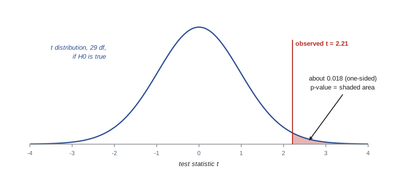
The clinic advertises that patients see a nurse within 15 minutes on average. Aisha suspects the true mean is longer. She takes a random sample of 30 visits and finds a mean of 17.9 minutes with a standard deviation of 7.2 minutes. The hypotheses are \(H_0: \mu = 15\) and \(H_a: \mu > 15\).
# One-sample t test: H0: mu = 15 vs Ha: mu > 15 minutes.
import math
from scipy import stats
n, xbar, s, mu0 = 30, 17.9, 7.2, 15
se = s / math.sqrt(n)
t = (xbar - mu0) / se
p_one = stats.t.sf(t, df=n - 1)          # area in the upper tail
print(f"SE = {se:.3f}, t = {t:.2f} with {n - 1} degrees of freedom")
print(f"one-sided p-value = {p_one:.4f}")
tstar = stats.t.ppf(0.975, df=n - 1)
print(f"95% CI for mu: ({xbar - tstar * se:.1f}, {xbar + tstar * se:.1f}) minutes")SE = 1.315, t = 2.21 with 29 degrees of freedom one-sided p-value = 0.0177 95% CI for mu: (15.2, 20.6) minutes
With a one-sided p-value of about 0.018, below 0.05, Aisha has moderate evidence that the mean wait exceeds 15 minutes. The confidence interval, roughly 15 to 21 minutes, tells the clinic how far off its advertised figure is likely to be, which is what it needs to decide whether to change staffing or change its advertising. A two-sided test at level \(\alpha\) and a confidence interval at level \(1 - \alpha\) always agree: the test rejects \(H_0\) exactly when the null value lies outside the interval.
Two kinds of errors
A test can go wrong in two ways. A Type I error rejects \(H_0\) when it is actually true: a false alarm, like convicting an innocent person or concluding that a useless drug works. A Type II error fails to reject \(H_0\) when it is false: a missed effect, like acquitting a guilty person or missing a drug that really helps. The probability of a Type I error equals the significance level \(\alpha\); choosing \(\alpha = 0.05\) means accepting a 5 percent chance of a false alarm when there is no effect.
| H0 is true | H0 is false | |
|---|---|---|
| Reject H0 | Type I error (false alarm), probability alpha | Correct decision (power) |
| Fail to reject H0 | Correct decision | Type II error (missed effect), probability beta |
The power of a test is the probability that it correctly rejects \(H_0\) when a particular alternative is true, equal to 1 minus the Type II error probability. Power rises with larger samples, larger true effects, less variable data and higher significance levels. A study with low power is likely to miss real effects, so researchers plan sample sizes to give power of 80 or 90 percent for the smallest effect they care about.
# Power by simulation: chance of detecting a true join rate of 0.25 (vs H0: 0.20) at alpha = 0.05.
import random, math
from statistics import NormalDist
random.seed(3)
zcrit = NormalDist().inv_cdf(0.95)          # one-sided test
def power(n, p_true, p0=0.20, reps=4000):
    hits = 0
    se0 = math.sqrt(p0 * (1 - p0) / n)
    for _ in range(reps):
        phat = sum(random.random() < p_true for _ in range(n)) / n
        hits += (phat - p0) / se0 >= zcrit
    return hits / reps
for n in (100, 200, 400, 800):
print(f"n = {n:3d}: power to detect p = 0.25 is about {power(n, 0.25):.2f}")n = 100: power to detect p = 0.25 is about 0.35 n = 200: power to detect p = 0.25 is about 0.52 n = 400: power to detect p = 0.25 is about 0.76 n = 800: power to detect p = 0.25 is about 0.96
With 100 invited members the café would detect a true improvement from 20 to 25 percent less than half the time, so a non-significant result would say almost nothing. With 800 it would detect the improvement almost every time. Planning sample size for adequate power before collecting data is one of the most valuable things a statistician does.
Statistical significance is not practical importance
With a very large sample, even tiny differences become statistically significant. If the café sent invitations to 200,000 members and the join rate rose from 20.0 to 20.3 percent, the p-value might be very small, but an increase of three-tenths of a percentage point may not be worth the cost of the program. Conversely, with a small sample, an important difference may fail to reach significance. Always report the size of the effect, ideally with a confidence interval, and judge its importance in context. A statistically significant result answers 'Is there evidence of some effect?', not 'Is the effect big enough to matter?'
Misuse: p-hacking and the replication crisis
If you test enough hypotheses, some will be significant by chance alone. At \(\alpha = 0.05\), testing 20 true null hypotheses produces, on average, one false positive. P-hacking is the practice, sometimes deliberate and often unconscious, of trying many analyses, outcomes, subgroups or data exclusions and reporting the ones that give p below 0.05. In the 2010s, large projects that tried to repeat published studies in psychology, medicine and economics found that many results, often far more than expected, did not replicate, a problem known as the replication crisis. Selective reporting, small samples and p-hacking were major causes.
In 2016 the American Statistical Association issued an unusual statement on p-values. Its main points were that p-values can indicate how incompatible the data are with a model, but they do not measure the probability that a hypothesis is true or that the data arose by chance alone; that scientific conclusions and business or policy decisions should not be based only on whether a p-value passes a threshold; that proper inference requires full reporting and transparency; and that a p-value does not measure the size or importance of an effect. Many fields now encourage pre-registered analysis plans, reporting of effect sizes with confidence intervals, and replication.
Worked problem
A complete test, with a reality check
A national survey finds that 30 percent of adults use public transit at least monthly. Lucas surveys a random sample of 250 city residents and finds 88 who do. Test whether the city's proportion differs from 30 percent at the 0.05 level, and comment on practical importance.
Show solution
- Hypotheses: H0: p = 0.30; Ha: p ≠ 0.30 (two-sided, since a difference in either direction matters).
- Conditions: random sample; np0 = 75 and n(1 - p0) = 175 are both at least 10.
- Statistic: p hat = 88/250 = 0.352; SE = sqrt(0.3 x 0.7 / 250) = 0.0290; z = (0.352 - 0.30) / 0.0290 = 1.79.
- p-value: two-sided area beyond 1.79 is about 2 x 0.0367 = 0.073.
- Conclusion: 0.073 > 0.05, so we fail to reject H0. The data give only weak evidence that the city differs from the national figure.
- Practical note: the estimated difference of about 5 percentage points might matter for transit planning, so a larger survey would be worthwhile; failing to reject does not show the proportions are equal.
Answer: z is about 1.79 and the p-value about 0.07, so H0 is not rejected at the 0.05 level, but a 5-point difference may still be practically important and deserves a larger sample.
Common mistakes
MistakeSaying the p-value is the probability that H0 is true.
InsteadThe p-value is the probability of data at least this extreme, assuming H0 is true.
MistakeConcluding that H0 is true when it is not rejected.
InsteadFailing to reject means the evidence was insufficient, not that H0 is proved.
MistakeWriting hypotheses about sample statistics, such as H0: p hat = 0.2.
InsteadHypotheses are about population parameters.
MistakeTreating any significant result as important.
InsteadReport and judge the effect size; large samples make tiny effects significant.
MistakeRunning many tests and reporting only the significant ones.
InsteadPlan analyses in advance and report all tests; multiple testing inflates false positives.
Summary and key terms
- A test assumes a null hypothesis of no effect and asks whether the data would be surprising if it were true.
- The p-value is the probability, under H0, of a result at least as extreme as the one observed; small p-values are evidence against H0.
- Compare the p-value with a significance level alpha chosen in advance; report the p-value itself.
- Use a z test for a proportion with the null standard error, and a t test with n - 1 degrees of freedom for a mean.
- Type I errors are false alarms (probability alpha); Type II errors are missed effects; power is the chance of detecting a real effect.
- Statistical significance is not practical importance, and p-hacking and selective reporting produce false discoveries.
- null hypothesis
- The claim of no effect or no difference that a test assumes in order to assess the evidence.
- alternative hypothesis
- The claim of an effect or difference that the test seeks evidence for.
- p-value
- The probability, assuming H0 is true, of a result at least as extreme as the one observed.
- significance level
- The threshold alpha below which a p-value leads to rejecting H0.
- statistically significant
- Having a p-value at or below the chosen significance level.
- test statistic
- A standardized measure of how far a sample result is from the null value.
- Type I error
- Rejecting a true null hypothesis.
- Type II error
- Failing to reject a false null hypothesis.
- power
- The probability of rejecting H0 when a specific alternative is true.
- p-hacking
- Trying many analyses and reporting those with small p-values.
Practice problems
Work each problem on paper first, then reveal the answer to check.
State hypotheses to test whether a coin is biased toward heads.
Show answer
H0: p = 0.5; Ha: p > 0.5, where p is the probability of heads.
A test gives p = 0.003. What do you conclude at alpha = 0.05?
Show answer
Reject H0: there is strong evidence against it.
A test gives p = 0.21. Does this prove H0 is true?
Show answer
No; the data are simply consistent with H0.
Find z for p hat = 0.56, p0 = 0.5, n = 400.
Show answer
SE = 0.025; z = 0.06/0.025 = 2.4.
In a drug trial, what would a Type II error mean?
Show answer
Concluding the drug has no effect when it actually works.
How can a researcher increase the power of a test?
Show answer
Use a larger sample, reduce variability or use a higher significance level.
A huge study finds a statistically significant 0.1-kilogram difference in weight loss. Is it important?
Show answer
Probably not practically important, despite being statistically significant.
Why are 20 tests at alpha = 0.05 likely to produce a false positive?
Show answer
Each true null has a 5 percent chance of rejection, so about one in 20 is expected by chance.
Lesson quiz · 5 questions
Score 60% or more to complete this lesson.
Create a free account to save your progress, take quizzes and earn a certificate.