
STAT-141 · Lesson 6 of 12 · 25 min
Correlation and regression
So far we have looked at one variable at a time. Many of the most interesting questions involve two: do students who study more score higher, does a store's sales rise with its advertising, do neighborhoods farther from downtown have longer commutes? This lesson covers the scatterplot, the correlation coefficient, the least-squares regression line used for prediction, and the reasons why an association between two variables does not, by itself, show that one causes the other.
Explanatory and response variables
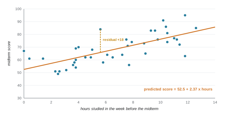
When we study how two quantitative variables are related, we often think of one as helping to explain or predict the other. The explanatory variable (also called the predictor or independent variable) goes on the horizontal axis, usually called x. The response variable (also called the outcome or dependent variable) goes on the vertical axis, called y. In Owen's study of 40 students in an introductory course, hours spent studying in the week before the midterm is the explanatory variable and the midterm score is the response.
Calling a variable explanatory does not mean it causes the response; it only reflects how we plan to use the data. Sometimes there is no natural direction at all, as with the heights of sisters, and then it does not matter which variable goes on which axis.
Scatterplots
A scatterplot shows the relationship between two quantitative variables measured on the same individuals. Each individual is one point, placed at its x and y values. Look at a scatterplot for four features. Direction: positive (larger x goes with larger y) or negative (larger x goes with smaller y). Form: roughly linear, curved, or clustered in groups. Strength: how closely the points follow the form. Unusual points: outliers that fall away from the overall pattern.
The correlation coefficient
The correlation coefficient, written r, measures the direction and strength of a linear relationship between two quantitative variables. It is computed from standardized values: \(r = \frac{1}{n-1}\sum \left(\frac{x_i - \bar{x}}{s_x}\right)\left(\frac{y_i - \bar{y}}{s_y}\right)\). When both values are above their means or both below, the product is positive; when one is above and the other below, it is negative. The average of these products tells us which tendency dominates.
Correlation has several important properties. It always falls between -1 and 1. Positive values indicate a positive association and negative values a negative one. Values near -1 or 1 mean the points lie close to a straight line; values near 0 mean a weak linear relationship. Correlation has no units and does not change if you change the units of either variable, say from minutes to hours or from dollars to euros. It does not distinguish between explanatory and response variables: the correlation of x with y equals the correlation of y with x.
Correlation also has important limits. It measures only linear relationships: a perfect curved relationship can have a correlation near zero. It is not resistant: one outlier can raise or lower it dramatically. And it is never a complete summary; always look at the scatterplot. The statistician Francis Anscombe made this point in 1973 with four small data sets that share the same means, standard deviations, correlation and regression line but look completely different when plotted.
| r | Description | What the scatterplot looks like |
|---|---|---|
| about 0.9 to 1 | Very strong positive | Points lie close to a rising line |
| about 0.5 to 0.8 | Moderate to strong positive | A clear rising pattern with noticeable scatter |
| about 0 | No linear relationship | A shapeless cloud, or a curve |
| about -0.5 to -0.8 | Moderate to strong negative | A clear falling pattern with scatter |
| about -0.9 to -1 | Very strong negative | Points lie close to a falling line |
The least-squares regression line
When a scatterplot shows a linear pattern, we can summarize it with a straight line and use the line to predict y from x. The line is written \(\hat{y} = a + bx\), where \(\hat{y}\) (read 'y hat') is the predicted response, b is the slope and a is the intercept. The slope tells you how much the predicted response changes when x increases by one unit; the intercept is the predicted value when x is zero, which may or may not have a sensible meaning.
Of all possible lines, the least-squares regression line is the one that makes the sum of the squared vertical distances from the points to the line as small as possible. Its slope and intercept have simple formulas in terms of summaries you already know: \(b = r \frac{s_y}{s_x}\) and \(a = \bar{y} - b\bar{x}\). The second formula shows that the line always passes through the point of means \((\bar{x}, \bar{y})\).
# Correlation and the least-squares line for study hours vs midterm score (40 invented students).
import random, statistics as st
random.seed(141)
hours = [round(random.uniform(0, 14), 1) for _ in range(40)]
score = [round(min(100, max(0, 52 + 2.6 * h + random.gauss(0, 8)))) for h in hours]
r = st.correlation(hours, score)
slope, intercept = st.linear_regression(hours, score)
print(f"mean hours {st.mean(hours):.2f}, mean score {st.mean(score):.2f}")
print(f"correlation r = {r:.3f}, r squared = {r * r:.3f}")
print(f"least-squares line: predicted score = {intercept:.1f} + {slope:.2f} x hours")
print(f"check b = r * sy / sx = {r * st.stdev(score) / st.stdev(hours):.2f}")
for h in (2, 8, 12):
print(f"predicted score for {h} hours: {intercept + slope * h:.1f}")mean hours 6.73, mean score 68.50 correlation r = 0.714, r squared = 0.510 least-squares line: predicted score = 52.5 + 2.37 x hours check b = r * sy / sx = 2.37 predicted score for 2 hours: 57.3 predicted score for 8 hours: 71.5 predicted score for 12 hours: 81.0
In context: each additional hour of study is associated with roughly 2 to 3 more marks on average, and a student who studied about 8 hours would be predicted to score around 72. The intercept, a predicted score for zero hours, is meaningful here because some students did study close to zero hours; in other problems the intercept is a mathematical device rather than a sensible prediction.
Residuals and r squared
A residual is the difference between an observed response and the value predicted by the line: residual = \(y - \hat{y}\). A positive residual means the point lies above the line (the student did better than predicted); a negative residual means it lies below. The least-squares line makes the residuals add to zero, and it makes the sum of their squares as small as possible.
The square of the correlation, \(r^2\), has a useful interpretation: it is the fraction of the variation in the response that is explained by the straight-line relationship with x. If \(r = 0.75\), then \(r^2 = 0.56\), so the regression on hours explains about 56 percent of the variation in scores; the other 44 percent is due to everything else, such as prior knowledge, sleep, test anxiety and luck.
Plotting the residuals against x is the best way to check whether a straight line is an appropriate model. A good residual plot looks like a horizontal band of random scatter around zero. A curved pattern means the relationship is not linear; a fan shape, with residuals spreading out as x increases, means the variability is not constant, which is common with money and counts.
# Residuals: positive above the line, negative below; they sum to zero.
import random, statistics as st
random.seed(141)
hours = [round(random.uniform(0, 14), 1) for _ in range(40)]
score = [round(min(100, max(0, 52 + 2.6 * h + random.gauss(0, 8)))) for h in hours]
b, a = st.linear_regression(hours, score)
res = [y - (a + b * x) for x, y in zip(hours, score)]
for x, y, e in list(zip(hours, score, res))[:4]:
    print(f"hours {x:4.1f}  score {y:3d}  predicted {a + b * x:5.1f}  residual {e:+6.1f}")
print(f"sum of residuals: {sum(res):.6f}")
print(f"largest positive residual {max(res):+.1f}, largest negative {min(res):+.1f}")hours 7.2 score 64 predicted 69.6 residual -5.6 hours 0.4 score 61 predicted 53.5 residual +7.5 hours 11.0 score 77 predicted 78.6 residual -1.6 hours 2.5 score 49 predicted 58.5 residual -9.5 sum of residuals: 0.000000 largest positive residual +18.2, largest negative -17.5
Prediction and extrapolation
Regression lines are made for prediction, but predictions are reliable only within the range of x values in the data. Using the line far outside that range is called extrapolation, and it is often badly wrong. Owen's students studied between 0 and 14 hours; the line predicts a score above 100 for 25 hours, which is impossible. Real relationships often bend or level off beyond the range we happened to observe. Business forecasts that extend a recent growth trend for decades are a common form of extrapolation.
Remember too that the regression of y on x is not the same as the regression of x on y. If you wanted to predict hours studied from a known score, you would need a different line, fitted by minimizing vertical distances in that direction.
Association is not causation
A strong correlation between two variables does not mean that one causes the other. Ice cream sales and drowning deaths rise and fall together, but both are driven by hot weather. Neighborhoods with more police officers may have more crime, because police are sent where crime is high. Countries with more televisions per person have longer life expectancies, because wealth drives both. In each case a lurking variable, one not included in the analysis, explains the association. A lurking variable that affects both the explanatory and response variables is a confounding variable, as in lesson 2.
Even when there is a causal link, it can run in the opposite direction from the one you expected, or in both directions. Only a randomized experiment provides direct evidence of cause. When experiments are impossible, researchers look for a consistent association across many studies and populations, a dose-response pattern, an association that holds after accounting for possible confounders, a plausible mechanism, and a cause that comes before its effect in time.
Simpson's paradox
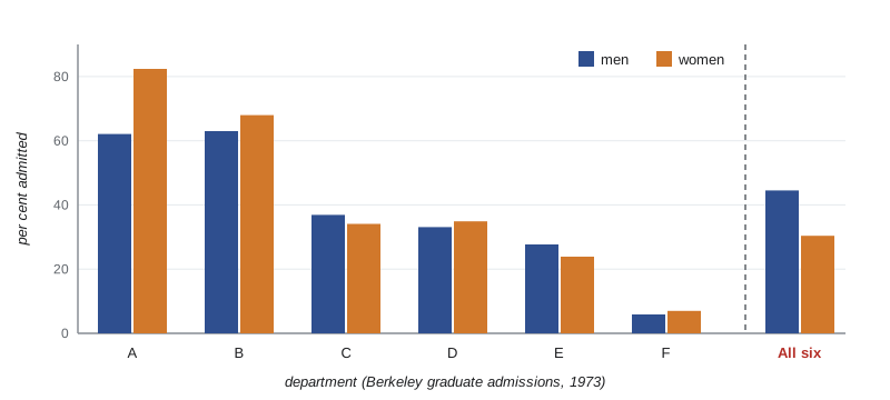
Lurking variables can do more than create a misleading association: they can reverse it. In 1973 the University of California, Berkeley, was concerned about possible bias against women in graduate admissions. Overall, about 44 percent of men who applied were admitted, compared with about 35 percent of women. But when statisticians looked department by department, most departments admitted women at a similar or higher rate than men. The explanation was that women applied more often to departments that admitted a small fraction of all applicants, while men applied more often to departments that admitted a large fraction. The department applied to was a lurking variable that reversed the direction of the comparison when the data were combined.
# Simpson's paradox: the six largest Berkeley departments, 1973 (applicants, percent admitted).
depts = {  # dept: (men applied, men admitted, women applied, women admitted)
    "A": (825, 512, 108, 89), "B": (560, 353, 25, 17), "C": (325, 120, 593, 202),
    "D": (417, 138, 375, 131), "E": (191, 53, 393, 94), "F": (373, 22, 341, 24)}
print("dept  men admitted  women admitted")
for d, (ma, mad, wa, wad) in depts.items():
    print(f"  {d}      {mad / ma:5.1%}        {wad / wa:5.1%}")
tm = sum(v[0] for v in depts.values()); tma = sum(v[1] for v in depts.values())
tw = sum(v[2] for v in depts.values()); twa = sum(v[3] for v in depts.values())
print(f"combined {tma / tm:5.1%} {twa / tw:5.1%} <- the direction reverses")dept men admitted women admitted A 62.1% 82.4% B 63.0% 68.0% C 36.9% 34.1% D 33.1% 34.9% E 27.7% 23.9% F 5.9% 7.0% combined 44.5% 30.4% <- the direction reverses
Women had the higher admission rate in four of the six departments, yet the combined rate for these six departments favors men by a wide margin. The reversal is not a trick of arithmetic: women mostly applied to the departments with low admission rates, such as C and E, while men mostly applied to A and B, where admission was easy. The lesson is to think about which variables might be lurking behind any comparison, and to compare like with like.
Worked problem
Interpreting a regression line
For 25 neighborhoods, Lucas regresses mean commute time (minutes) on distance from downtown. The line is predicted commute = 11.2 + 1.85 x distance, with r = 0.83. Interpret the slope, intercept and r squared, predict the commute for a neighborhood 10 units from downtown, and say whether you could use the line for a town 60 units away when the data cover 1 to 20.
Show solution
- Slope: each additional unit of distance is associated with about 1.85 more minutes of mean commute time.
- Intercept: a neighborhood right downtown would be predicted to have an average commute of about 11 minutes, which is plausible because residents still travel to work within the core.
- r squared = 0.83 squared = 0.69, so distance explains about 69 percent of the variation in mean commute times across neighborhoods.
- Prediction at 10: 11.2 + 1.85 x 10 = 29.7 minutes.
- At 60, far beyond the data range of 1 to 20, the prediction would be extrapolation; commuting patterns (highways, remote work) may differ, so the line should not be trusted there.
Answer: Each unit of distance adds about 1.85 minutes, distance explains about 69 percent of the variation, the prediction at 10 is about 29.7 minutes, and predicting at 60 would be unreliable extrapolation.
Common mistakes
MistakeConcluding that x causes y because the correlation is strong.
InsteadConsider lurking and confounding variables; only randomized experiments show cause directly.
MistakeUsing correlation to describe a curved relationship.
InsteadCorrelation measures only linear association; look at the scatterplot.
MistakeIgnoring an outlier that drives the correlation or the line.
InsteadCheck how the results change with and without the unusual point, and investigate it.
MistakePredicting far outside the range of the data.
InsteadAvoid extrapolation; relationships may change beyond the observed range.
MistakeCombining groups without checking for a lurking variable.
InsteadCompare within groups too; Simpson's paradox can reverse a combined comparison.
Summary and key terms
- A scatterplot shows the direction, form, strength and unusual points of a relationship between two quantitative variables.
- The correlation r measures the direction and strength of a linear relationship, lies between -1 and 1, has no units and is not resistant.
- The least-squares line y hat = a + bx minimizes the sum of squared residuals, with b = r sy/sx, and passes through the point of means.
- r squared is the fraction of the variation in y explained by the linear relationship with x.
- Residual plots check whether a line is appropriate; extrapolation beyond the data is unreliable.
- Association is not causation, and lurking variables can even reverse an association (Simpson's paradox).
- explanatory variable
- The variable used to explain or predict another, plotted on the horizontal axis.
- response variable
- The outcome variable, plotted on the vertical axis.
- scatterplot
- A graph of two quantitative variables with one point per individual.
- correlation
- A number between -1 and 1 measuring the direction and strength of a linear relationship.
- least-squares regression line
- The line that minimizes the sum of squared vertical distances from the points.
- slope
- The change in the predicted response for a one-unit increase in the explanatory variable.
- residual
- An observed response minus the response predicted by the regression line.
- r squared
- The fraction of the variation in the response explained by the regression on x.
- extrapolation
- Using a regression line to predict outside the range of the data.
- lurking variable
- A variable not included in an analysis that affects the relationship between the variables studied.
- Simpson's paradox
- A reversal in the direction of an association when data from several groups are combined.
Practice problems
Work each problem on paper first, then reveal the answer to check.
A scatterplot of house size and price rises from left to right with points close to a line. Describe the relationship.
Show answer
Strong, positive and linear.
If r = -0.6, what is r squared and what does it mean?
Show answer
0.36: about 36 percent of the variation in y is explained by the linear relationship with x.
Does changing temperature from Celsius to Fahrenheit change the correlation with ice cream sales?
Show answer
No; correlation has no units and is unchanged by linear changes of scale.
A line is y hat = 20 + 3x. Predict y when x = 5 and find the residual if the observed y is 31.
Show answer
Predicted 35; residual 31 - 35 = -4.
Given r = 0.8, sx = 2 and sy = 10, find the slope.
Show answer
b = 0.8 x 10 / 2 = 4.
Towns with more churches have more bars. Suggest a lurking variable.
Show answer
Population size.
What pattern in a residual plot suggests a straight line is a poor model?
Show answer
A curved pattern (or a fan shape showing changing spread).
In one sentence, what is Simpson's paradox?
Show answer
An association within every group reverses when the groups are combined, because of a lurking variable.
Lesson quiz · 5 questions
Score 60% or more to complete this lesson.
Create a free account to save your progress, take quizzes and earn a certificate.