
STAT-141 · Lesson 2 of 12 · 28 min
Collecting data: sampling and study design
A statistical conclusion can never be better than the data behind it. The cleverest analysis cannot rescue a sample that left out half the population or an experiment in which the treatment group was healthier to begin with. This lesson is about producing data that deserve to be analyzed: choosing samples that represent a population, writing survey questions that measure what you intend, and designing comparisons that can support claims about cause and effect.
Levels of measurement
Before collecting anything, decide what kind of values each variable will take, because that decides which summaries and methods make sense later. Statisticians describe four levels of measurement. Nominal variables are categories with no order, such as travel mode or blood type. Ordinal variables are categories with a natural order but uneven or unknown spacing, such as satisfaction ratings from very dissatisfied to very satisfied, or education level. Interval variables are numerical with equal spacing but no true zero, such as temperature in degrees Celsius or Fahrenheit, where 20 degrees is not twice as hot as 10. Ratio variables are numerical with a true zero, such as income, weight, commute time or number of visits, where ratios make sense: a 40-minute commute is twice as long as a 20-minute one.
| Level | Order? | Equal spacing? | True zero? | Examples | Sensible summaries |
|---|---|---|---|---|---|
| Nominal | No | No | No | Travel mode, blood type, favorite café | Counts, percentages, mode |
| Ordinal | Yes | No | No | Satisfaction rating, pain scale, education level | Counts, median, percentiles |
| Interval | Yes | Yes | No | Temperature in °C or °F, calendar year | Mean, standard deviation, differences |
| Ratio | Yes | Yes | Yes | Income, weight, commute time, visits | All of the above, plus ratios |
In practice, analysts often treat ordinal rating scales as if they were interval, for example by averaging satisfaction scores from 1 to 5. That is usually harmless for rough comparisons, but you should know you are making an assumption, and medians or percentages in each category are often more honest summaries of ordinal data.
Observational studies and experiments
There are two fundamentally different ways to collect data about a relationship. In an observational study you measure individuals as they are, without trying to influence them: you survey residents about their commute and their stress levels, or you compare the health records of people who chose to get a flu shot with those who did not. In an experiment you deliberately impose a treatment on individuals to see how they respond: you randomly give half of a group of customers a discount coupon and compare their spending with the other half.
The difference matters because observational studies can show that two variables are associated, but they struggle to show that one causes the other. People who choose to get flu shots may also wash their hands more, see doctors more often and have higher incomes, and any of those could explain why they have fewer hospital visits. A variable that is related to both the explanatory variable and the response, and so muddies the comparison, is called a confounding variable. Well-designed experiments get around confounding by random assignment, which we discuss below.
Observational studies are still valuable. They are often the only ethical or practical option: you cannot randomly assign people to smoke or to live in poverty. They can study large populations over long periods, and careful designs can make causal conclusions more convincing. The famous studies linking smoking to lung cancer were observational, but they were large, consistent across many populations, showed a dose-response pattern and had a plausible biological mechanism, which together built a strong case.
Sampling: why not just ask everyone?
A census tries to collect data from every member of the population. Censuses are expensive and slow, and even national censuses miss some people. Most of the time we take a sample instead. Surprisingly, a well-chosen sample of a thousand or so people can describe a population of millions with useful precision, because what matters most is how the sample was chosen and how large it is, not what fraction of the population it covers. A poorly chosen sample of a million can be worse than a good sample of a thousand.
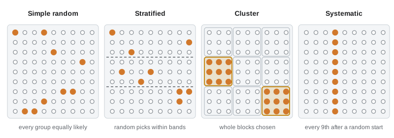
The key idea is randomness. In a simple random sample (SRS) of size n, every possible group of n individuals from the population has the same chance of being the sample. Choosing by chance removes the influence of the person doing the choosing, who might, consciously or not, favor people who are easy to reach, friendly-looking or similar to themselves. Random selection also makes it possible to calculate how much sample results are likely to vary, which is the basis of margins of error.
# Drawing a simple random sample of 10 households from a list of 2,000.
import random
random.seed(141)
population = list(range(1, 2001))          # household ID numbers on the city's list
sample = sorted(random.sample(population, 10))
print("simple random sample of household IDs:", sample)
# A second draw gives a different sample: sampling variability
print("a second random sample: ", sorted(random.sample(population, 10)))simple random sample of household IDs: [62, 364, 947, 973, 1060, 1175, 1189, 1429, 1595, 1606] a second random sample: [4, 26, 551, 703, 843, 1150, 1334, 1404, 1843, 1895]
Software makes random selection easy, but you still need a list of the population to choose from, called a sampling frame. The frame might be a list of addresses, a membership roster or a set of phone numbers. If the frame leaves out part of the population, such as people without a fixed address or households without a landline, no amount of randomness will bring them back. This is called undercoverage.
Other random sampling designs
Simple random samples are not always practical or the most efficient. Several other probability sampling designs are widely used, all of which use chance but organize it differently.
A stratified random sample first divides the population into groups called strata that are similar within themselves, such as neighborhoods, age groups or store regions, and then takes a separate simple random sample within each stratum. Stratifying guarantees that every group is represented and usually gives more precise estimates, especially when the strata differ from each other. National surveys almost always stratify by region.
A cluster sample divides the population into many groups called clusters, often geographic, randomly selects some clusters and then measures everyone, or a random sample, within the chosen clusters. For example, the food bank might randomly select 20 city blocks and interview every household on them. Cluster sampling is cheaper because interviewers travel less, but it is usually less precise than a simple random sample of the same size because people within a cluster tend to resemble each other.
A systematic sample chooses a random starting point and then takes every kth individual from a list, such as every 20th customer through the door. It is easy to carry out and works well as long as the list has no repeating pattern that lines up with k.
| Design | How it works | Main advantage | Main drawback |
|---|---|---|---|
| Simple random sample | Every possible sample of size n equally likely | Simple to analyze; unbiased | Needs a complete list; may miss small groups by chance |
| Stratified | Separate random samples within strata | Every group represented; more precise | Need to know each individual's stratum in advance |
| Cluster | Randomly choose whole groups (clusters) | Cheaper fieldwork; no full list of individuals needed | Less precise for the same sample size |
| Systematic | Every kth individual after a random start | Very easy in the field | Biased if the list has a pattern matching k |
How samples go wrong
Bias is a systematic tendency for a study to favor certain outcomes, so that the results miss the truth in a consistent direction. Unlike random sampling variability, bias does not shrink when you collect more data. Several kinds of bias are especially common.
Convenience sampling chooses whoever is easiest to reach: shoppers at one mall on a weekday afternoon, students in one class, your social media followers. Such samples rarely represent the wider population. Voluntary response sampling lets people decide for themselves whether to take part, as in call-in shows, website polls and many online reviews. People with strong opinions, especially negative ones, are much more likely to respond, so voluntary response samples are usually badly biased.
Non-response bias occurs when people chosen for a sample cannot be reached or refuse to answer, and those who do respond differ from those who do not. Response rates for telephone surveys have fallen to the single digits in many countries, so pollsters work hard to adjust for who is missing, using a technique called weighting. Response bias occurs when people answer inaccurately: they may round, misremember, give the answer they think is socially acceptable (under-reporting alcohol use or over-reporting voting), or react to the interviewer.
# Simulating voluntary response bias: true satisfaction vs who chooses to answer.
import random
random.seed(7)
customers = [random.choice([1, 2, 3, 4, 5]) for _ in range(10000)]   # satisfaction 1..5, uniform here
true_mean = sum(customers) / len(customers)
# Very unhappy (1) and very happy (5) customers are far more likely to respond
respond_prob = {1: 0.40, 2: 0.08, 3: 0.05, 4: 0.08, 5: 0.25}
responders = [c for c in customers if random.random() < respond_prob[c]]
print(f"true mean satisfaction of all customers: {true_mean:.2f}")
print(f"responders: {len(responders)} of {len(customers)}")
print(f"mean among responders:                   {sum(responders) / len(responders):.2f}")
print(f"share of responders rating 1 (very unhappy): {responders.count(1) / len(responders):.0%}")true mean satisfaction of all customers: 2.96 responders: 1683 of 10000 mean among responders: 2.55 share of responders rating 1 (very unhappy): 49%
The simulation shows how voluntary response distorts results. Even though satisfaction is spread evenly among all customers, the responders are dominated by the very unhappy and the very happy, so the share of extreme ratings is greatly exaggerated. Online review sites show this pattern: ratings tend to pile up at one and five stars.
Writing good survey questions
How you ask a question can change the answer dramatically. Leading questions push respondents toward an answer: 'Don't you agree that the city should improve its unreliable bus service?' Loaded words carry emotional weight: 'welfare' and 'assistance to the poor' can draw quite different levels of support for the same program. Double-barrelled questions ask two things at once: 'Are you satisfied with the price and quality of our coffee?' Questions should be short, neutral, ask one thing and offer balanced answer choices.
Question order matters too. Asking about recent crime before asking how safe people feel can lower reported feelings of safety. Answer options can anchor responses: offering income brackets that start at a very high amount can make people report higher incomes. Professional survey designers test questions on small groups before a full survey, a step called a pilot or pretest.
| Problem | Poor wording | Better wording |
|---|---|---|
| Leading | Wouldn't you agree that the new bike lanes are a waste of money? | Do you support or oppose the new bike lanes on Main Street? |
| Double-barrelled | How satisfied are you with our prices and service? | Ask two questions: one about prices and one about service |
| Jargon | Do you favor TOD near LRT stations? | Do you favor building housing near the new light-rail stations? |
| Unbalanced options | Excellent / Very good / Good / Fair | Very good / Good / Neither / Poor / Very poor |
| Vague time frame | Do you exercise regularly? | On how many days in the past 7 days did you exercise for at least 30 minutes? |
Polls and margins of error
Opinion polls are the samples most people see. A typical national poll surveys 1,000 to 2,000 adults and reports a margin of error of around 2 to 3 percentage points, 19 times out of 20. That phrase means that if the poll were repeated many times with fresh random samples, about 95 percent of the resulting intervals would contain the true population percentage. Lesson 10 explains where this comes from. The margin of error covers only random sampling variability; it does not account for bias from non-response, poor question wording or people changing their minds.
Polls are generally useful but not perfect. Studies of election polling in Canada, the United States and elsewhere find that final pre-election polls usually come within a few percentage points of the result, but they sometimes miss in the same direction across many firms at once, which suggests shared bias rather than bad luck. Analysts therefore look at averages of many polls, check each pollster's methods, and treat close races as genuinely uncertain.
Designing experiments
An experiment imposes treatments on experimental units (called subjects or participants when they are people) and measures a response. Three principles make an experiment trustworthy. Control means comparing the treatment with a control group that does not receive it, or receives a placebo or the standard treatment, so that other influences affect both groups alike. Randomization means using chance to assign units to groups, which balances confounding variables, known and unknown, on average. Replication means using enough units in each group that chance differences between groups are small.
Back at the café chain, Owen proposes an experiment: among 600 loyalty members who have not yet activated the new app feature, randomly choose 300 to receive an invitation and a bonus offer, and leave the other 300 as a control group. After two months, compare the average number of visits. Because chance alone decided who got the invitation, the two groups should be similar in habits, income, distance from a café and everything else, so a clear difference in visits can be attributed to the invitation.
# Random assignment of 600 customers to treatment and control groups.
import random
random.seed(2026)
customers = [f"C{i:03d}" for i in range(1, 601)]
random.shuffle(customers)
treatment, control = customers[:300], customers[300:]
print("first five in treatment:", treatment[:5])
print("first five in control:  ", control[:5])
# Randomization balances background variables on average: check a made-up one
distance = {c: random.uniform(0.2, 8.0) for c in customers}   # km from nearest cafe
avg = lambda g: sum(distance[c] for c in g) / len(g)
print(f"average distance, treatment: {avg(treatment):.2f} km; control: {avg(control):.2f} km")first five in treatment: ['C227', 'C201', 'C172', 'C087', 'C543'] first five in control: ['C057', 'C111', 'C520', 'C294', 'C288'] average distance, treatment: 4.24 km; control: 4.16 km
Two further refinements are common. Blinding means that participants, and ideally the people measuring the response, do not know who is in which group, which prevents expectations from shaping the results. In medical trials, double-blind designs with a placebo are standard because of the placebo effect: people often feel better after receiving any treatment they believe might help. Blocking means grouping similar units first, for example by store or by age group, and then randomizing within each block, which removes the block-to-block variation from the comparison. A matched-pairs design is the simplest kind of blocking: each person receives both treatments in random order, or pairs of similar people are split between the treatments.
Worked problem
Spotting the design and its weakness
A clinic wants to know whether text-message reminders reduce missed appointments. In January it sends no reminders and 14 percent of appointments are missed. In February it sends reminders to everyone and 9 percent are missed. Is this an experiment? What is the main weakness, and how could the clinic do better?
Show solution
- Treatments were imposed (reminders were sent), but there was no randomly assigned control group at the same time.
- January and February differ in weather, holidays, illness and staffing, any of which could change missed appointments; these are confounding variables.
- Better design: during the same months, randomly assign each patient (or each appointment) to receive or not receive a reminder, and compare missed-appointment rates between the two groups.
- Randomization balances weather, season and patient characteristics between groups, so a difference can be credited to the reminders.
Answer: It is a before-and-after comparison without a concurrent randomized control, so month-to-month differences confound the result; a randomized comparison in the same period is better.
Common mistakes
MistakeBelieving a very large sample automatically represents the population.
InsteadCheck how individuals were chosen; a biased method stays biased however large the sample.
MistakeTreating an online or call-in poll as a random sample.
InsteadVoluntary response samples overrepresent strong opinions and cannot be generalized.
MistakeConcluding cause and effect from an observational study.
InsteadLook for confounding variables; only randomized experiments give direct evidence of cause.
MistakeComparing a treated group with an untreated group chosen by convenience.
InsteadAssign treatments at random so the groups are alike apart from the treatment.
MistakeThinking the margin of error covers all possible errors in a poll.
InsteadIt covers random sampling variability only, not non-response, wording or coverage bias.
Summary and key terms
- Levels of measurement (nominal, ordinal, interval, ratio) decide which summaries are sensible.
- Observational studies measure individuals as they are and can show association; experiments impose treatments and, with randomization, can show cause.
- Random sampling removes selection bias and lets us measure sampling variability.
- Stratified, cluster and systematic samples organize randomness differently, trading precision against cost.
- Convenience, voluntary response, undercoverage, non-response and response bias distort results and do not shrink with larger samples.
- Good experiments use control, randomization and replication, and often blinding and blocking.
- observational study
- A study that measures individuals without influencing them.
- experiment
- A study that deliberately imposes treatments and measures responses.
- confounding variable
- A variable related to both the explanatory variable and the response that distorts their apparent relationship.
- simple random sample
- A sample chosen so that every possible group of n individuals has the same chance of selection.
- sampling frame
- The list of individuals from which a sample is drawn.
- stratified random sample
- Separate simple random samples taken within groups of similar individuals.
- cluster sample
- A sample formed by randomly selecting whole groups and measuring individuals within them.
- bias
- A systematic tendency for a study to miss the truth in a consistent direction.
- non-response bias
- Bias that arises when those who do not respond differ from those who do.
- random assignment
- Using chance to decide which units receive which treatment.
- placebo effect
- Improvement that occurs because participants believe they are being treated.
- blocking
- Grouping similar units and randomizing treatments within each group.
Practice problems
Work each problem on paper first, then reveal the answer to check.
Classify the level of measurement: year of birth, number of pets, T-shirt size (S, M, L), eye color.
Show answer
Interval; ratio; ordinal; nominal.
A study compares heart disease rates in people who choose to eat oatmeal with those who do not. Experiment or observational study?
Show answer
Observational: the researchers did not assign oatmeal.
Name a possible confounding variable in the oatmeal study.
Show answer
Overall diet quality, exercise or income, which may relate to both oatmeal eating and heart health.
A school takes a random sample of 10 students from each grade. What design is this?
Show answer
Stratified random sampling with grades as strata.
Why does a larger voluntary online poll not fix its bias?
Show answer
Bias comes from who chooses to respond, which more responses of the same kind do not change.
Rewrite the double-barrelled question "Is the library clean and quiet?"
Show answer
Ask separately: "Is the library clean?" and "Is the library quiet?"
What are the three basic principles of experimental design?
Show answer
Control, randomization and replication.
In a taste test of two coffees, why should tasters not know which brand they are drinking?
Show answer
Blinding prevents brand expectations from influencing their ratings.
Lesson quiz · 5 questions
Score 60% or more to complete this lesson.
Create a free account to save your progress, take quizzes and earn a certificate.