
STAT-141 · Lesson 4 of 12 · 24 min
Describing data with numbers
Graphs show the overall pattern; numerical summaries pin it down. A food bank planning next month's orders needs a number for typical weekly demand and a number for how much demand varies. This lesson covers measures of center (mean, median and mode), measures of spread (range, interquartile range and standard deviation), the five-number summary and boxplot, z-scores, and weighted means, including the price indexes that measure inflation.
The food bank data
The food bank serves households in several neighborhoods. Lucas collects the number of households served each week for the past 52 weeks, and the amount each of 200 visiting households said it spends on groceries in a typical week. Both variables are quantitative; weekly visits are roughly symmetric, while grocery spending is skewed to the right, with a few large households spending much more than most.
Measures of center
The mean is the ordinary average: add up the values and divide by how many there are. If the values are \(x_1, x_2, \ldots, x_n\), the sample mean is \(\bar{x} = \frac{1}{n}\sum x_i\). The mean uses every value, which is both its strength and its weakness: a single very large value can pull it a long way.
The median is the middle value when the data are put in order. With an odd number of values it is the middle one; with an even number it is the average of the two middle ones. Half the data fall at or below the median and half at or above. The median depends only on the order of the values, so it is resistant to outliers and extreme values: making the largest value ten times bigger leaves the median unchanged.
The mode is the most common value. It is the only measure of center that works for nominal categorical data (the most common travel mode is car), but for quantitative data it is often unhelpful, because continuous values may never repeat exactly.
# Mean, median and mode of weekly grocery spending for 9 households (dollars).
import statistics as st
spend = [85, 92, 110, 110, 124, 131, 140, 168, 420]
print("mean:  ", round(st.mean(spend), 2))
print("median:", st.median(spend))
print("mode:  ", st.mode(spend))
# Without the one large household
print("mean without 420:  ", round(st.mean(spend[:-1]), 2))
print("median without 420:", st.median(spend[:-1]))mean: 153.33 median: 124 mode: 110 mean without 420: 120 median without 420: 117.0
The relationship between the mean and the median tells you about shape. In a symmetric distribution they are close together. In a right-skewed distribution the long upper tail pulls the mean above the median; in a left-skewed distribution the mean falls below the median. That is why reports on income and house prices usually quote the median: the mean is dragged upward by a small number of very high values and overstates what a typical household earns or pays.
| Measure | How to find it | Resistant to outliers? | Best used for |
|---|---|---|---|
| Mean | Sum of values divided by n | No | Roughly symmetric quantitative data; totals and averages per person |
| Median | Middle value in order | Yes | Skewed data such as income, prices and waiting times |
| Mode | Most common value | Yes | Categorical data; peaks in a distribution |
Measures of spread
Two neighborhoods can have the same average grocery spending but very different variation, and for planning, variation often matters more than the average. The simplest measure of spread is the range, the largest value minus the smallest. It is easy to compute but depends entirely on the two most extreme values, so a single outlier can change it enormously.
Quartiles divide the ordered data into four parts. The first quartile, Q1, is the median of the lower half of the data; the third quartile, Q3, is the median of the upper half. About a quarter of the values fall below Q1 and a quarter above Q3. The interquartile range, IQR = Q3 - Q1, is the spread of the middle half of the data. Like the median, it is resistant to outliers. Different software packages use slightly different rules for quartiles, so you may see small differences in their answers; they all agree on the idea.
The standard deviation measures the typical distance of the values from their mean. To compute it, find each value's deviation from the mean, \(x_i - \bar{x}\); square the deviations so that positive and negative ones do not cancel; add them up; divide by \(n - 1\); and take the square root. In symbols, \(s = \sqrt{\frac{1}{n-1}\sum (x_i - \bar{x})^2}\). The quantity before the square root, \(s^2\), is called the variance. Dividing by \(n - 1\) rather than n makes the sample variance a better estimate of the population variance; you will see why in lesson 9. The standard deviation is in the same units as the data, which makes it easy to interpret: a standard deviation of 30 dollars means that households typically differ from the mean by roughly 30 dollars.
# Standard deviation step by step for five weekly visit counts.
import math, statistics as st
x = [212, 198, 225, 240, 205]          # households served in five weeks
mean = sum(x) / len(x)
dev = [v - mean for v in x]
sq = [d * d for d in dev]
var = sum(sq) / (len(x) - 1)
print("mean:", mean)
print("deviations:", [round(d, 1) for d in dev], " (they sum to", round(sum(dev), 10), ")")
print("squared deviations:", [round(s, 1) for s in sq])
print(f"variance = {sum(sq):.1f} / {len(x) - 1} = {var:.1f}")
print(f"standard deviation = sqrt({var:.1f}) = {math.sqrt(var):.2f}")
print("check with statistics.stdev:", round(st.stdev(x), 2))mean: 216.0 deviations: [-4.0, -18.0, 9.0, 24.0, -11.0] (they sum to 0.0 ) squared deviations: [16.0, 324.0, 81.0, 576.0, 121.0] variance = 1118.0 / 4 = 279.5 standard deviation = sqrt(279.5) = 16.72 check with statistics.stdev: 16.72
The standard deviation is zero only when all values are identical, and it grows as values spread out. Like the mean, it is strongly affected by outliers and skewness, because squaring gives extreme deviations a lot of weight. A common pairing rule follows: report the mean and standard deviation for roughly symmetric data without outliers, and the median and IQR (or the five-number summary) for skewed data or data with outliers.
The five-number summary and boxplots
The five-number summary consists of the minimum, Q1, the median, Q3 and the maximum. Together they describe the center, the spread of the middle half, and the extremes. A boxplot draws the five-number summary: a box from Q1 to Q3 with a line at the median, and whiskers extending to the smallest and largest values that are not outliers.
A common rule identifies outliers as values more than 1.5 IQR below Q1 or above Q3. These limits are sometimes called fences. In a modified boxplot, which most software draws by default, points beyond the fences are plotted individually and the whiskers stop at the most extreme values inside them. The rule is only a screening tool: it flags values worth a second look, not values that must be wrong.
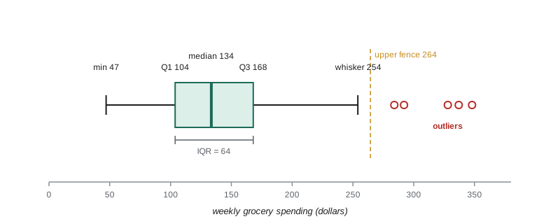
# Five-number summary and the 1.5 x IQR outlier rule for 200 invented spending values.
import random, statistics as st
random.seed(41)
spend = sorted(round(random.lognormvariate(4.85, 0.38)) for _ in range(200))
q1, med, q3 = st.quantiles(spend, n=4, method="inclusive")
iqr = q3 - q1
lo_fence, hi_fence = q1 - 1.5 * iqr, q3 + 1.5 * iqr
print("five-number summary:", spend[0], round(q1, 1), round(med, 1), round(q3, 1), spend[-1])
print(f"IQR = {iqr:.1f}; fences at {lo_fence:.1f} and {hi_fence:.1f}")
out = [v for v in spend if v < lo_fence or v > hi_fence]
print("values flagged as outliers:", out)
print(f"mean {st.mean(spend):.1f} vs median {med:.1f}: mean is higher, as expected for right skew")five-number summary: 47 103.8 133.5 168.0 348 IQR = 64.2; fences at 7.4 and 264.4 values flagged as outliers: [284, 292, 328, 337, 348] mean 141.9 vs median 133.5: mean is higher, as expected for right skew
Side-by-side boxplots are one of the best ways to compare a quantitative variable across groups. Lucas draws boxplots of grocery spending for households with one, two, three and four or more members; the medians rise with household size, the boxes overlap, and the largest households show the most spread. In a glance you see both the pattern and its variability.
Standardizing with z-scores
How unusual is a particular value? The answer depends on both the center and the spread of its distribution. A z-score measures how many standard deviations a value lies above or below the mean: \(z = \frac{x - \bar{x}}{s}\). A positive z-score means above the mean, a negative one below it. A household spending 220 dollars a week when the mean is 140 and the standard deviation is 40 has \(z = (220 - 140)/40 = 2\): it spends two standard deviations more than average.
Z-scores let you compare values measured on different scales. Suppose Owen scores 78 on a statistics test with mean 70 and standard deviation 5, and 85 on an economics test with mean 80 and standard deviation 10. His z-scores are 1.6 and 0.5, so relative to his classmates he did much better in statistics, even though his raw score was lower. In lesson 5, z-scores connect to the normal distribution and to percentiles.
Weighted means and price indexes
Sometimes values deserve different weights. A course grade in which the final exam counts 50 percent, the midterm 30 percent and assignments 20 percent is a weighted mean: \(\bar{x}_w = \frac{\sum w_i x_i}{\sum w_i}\). A student with 72 on the final, 85 on the midterm and 90 on assignments has a weighted mean of \((0.5 \times 72) + (0.3 \times 85) + (0.2 \times 90) = 79.5\), lower than the simple average of 82.3 because the weakest mark carries the most weight.
A consumer price index is a weighted mean on a large scale. It tracks the cost of a fixed basket of goods and services that represents what households buy. Each category, such as shelter, food, transportation and clothing, gets a weight equal to its share of typical spending, and the index combines the price changes in each category using those weights. Because shelter takes a much larger share of household budgets than clothing, a 10 percent rise in rents moves the index far more than a 10 percent rise in shirt prices.
In the United States, the Bureau of Labor Statistics publishes the CPI monthly; the most widely quoted version, the CPI for All Urban Consumers (CPI-U), uses 1982 to 1984 as the base period set equal to 100. The basket weights are updated every year from the Consumer Expenditure Surveys. Shelter is the largest component, at roughly a third of the index. The Federal Reserve's 2 percent inflation goal is defined in terms of a related measure, the personal consumption expenditures price index, but the CPI remains the best-known inflation figure.
# A simplified price index: weighted average of price changes in four categories (invented).
weights = {"shelter": 0.30, "food": 0.17, "transportation": 0.18, "other": 0.35}
price_change = {"shelter": 0.052, "food": 0.031, "transportation": -0.012, "other": 0.021}   # one-year % change
for k in weights:
    print(f"{k:<15} weight {weights[k]:.2f}  price change {price_change[k]:+.1%}  contribution {weights[k] * price_change[k]:+.2%}")
inflation = sum(weights[k] * price_change[k] for k in weights)
simple = sum(price_change.values()) / len(price_change)
print(f"weighted inflation: {inflation:.2%} (unweighted average of changes: {simple:.2%})")shelter weight 0.30 price change +5.2% contribution +1.56% food weight 0.17 price change +3.1% contribution +0.53% transportation weight 0.18 price change -1.2% contribution -0.22% other weight 0.35 price change +2.1% contribution +0.73% weighted inflation: 2.61% (unweighted average of changes: 2.30%)
Price indexes are also how you compare money across time. To express a past amount in today's dollars, multiply it by the ratio of today's index to the past index. If the index was 120 when your parents bought a car for 18,000 dollars and is 160 today, that price is equivalent to \(18000 \times 160/120 = 24000\) of today's dollars. Wages, rents and prices compared over long periods should almost always be adjusted for inflation in this way.
Worked problem
Choosing summaries
The clinic records how many minutes 11 patients wait: 4, 7, 8, 9, 10, 12, 12, 14, 18, 22, 95. Find the mean, median, quartiles, IQR and fences, and decide which summaries to report.
Show solution
- Mean: the total is 211, so the mean is 211 / 11 = 19.2 minutes.
- Median: the 6th of 11 ordered values, 12 minutes.
- Quartiles: the lower half (4, 7, 8, 9, 10) has median Q1 = 8; the upper half (12, 14, 18, 22, 95) has median Q3 = 18. IQR = 18 - 8 = 10.
- Fences: 8 - 15 = -7 and 18 + 15 = 33, so 95 is flagged as an outlier.
- Because the distribution is skewed with an outlier, the median (12) and IQR (10) describe a typical wait better than the mean (19.2), which the 95-minute wait pulls up.
Answer: Report the median of 12 minutes and IQR of 10, note the 95-minute outlier, and avoid the mean of 19.2, which overstates the typical wait.
Common mistakes
MistakeReporting the mean income or house price as "typical".
InsteadUse the median for skewed data; the mean is pulled up by a few very large values.
MistakeDividing by n instead of n - 1 for a sample standard deviation.
InsteadThe sample standard deviation divides the sum of squared deviations by n - 1.
MistakeTreating every point beyond the 1.5 IQR fences as an error.
InsteadThe rule flags values to investigate; many are genuine.
MistakeComparing raw scores from tests with different means and spreads.
InsteadConvert to z-scores to compare relative standing.
MistakeComparing dollar amounts from different decades directly.
InsteadAdjust for inflation with a price index first.
Summary and key terms
- The mean uses every value but is pulled by outliers and skew; the median is resistant; the mode is the most common value.
- In right-skewed data the mean exceeds the median.
- The range, IQR and standard deviation measure spread; the IQR is resistant, the standard deviation is not.
- The five-number summary underlies the boxplot, and the 1.5 IQR rule flags possible outliers.
- A z-score states how many standard deviations a value is from the mean and allows comparisons across scales.
- Weighted means combine values of different importance; a consumer price index is a weighted mean of price changes.
- mean
- The sum of the values divided by their number.
- median
- The middle value of the ordered data.
- resistant measure
- A summary that is not strongly affected by extreme values.
- quartiles
- Values that divide ordered data into four equal parts; Q1 and Q3 bound the middle half.
- interquartile range
- Q3 minus Q1, the spread of the middle half of the data.
- standard deviation
- The square root of the variance, measuring typical distance from the mean.
- variance
- The sum of squared deviations from the mean divided by n - 1.
- five-number summary
- The minimum, Q1, median, Q3 and maximum.
- z-score
- The number of standard deviations a value lies above or below the mean.
- weighted mean
- An average in which each value is multiplied by a weight reflecting its importance.
- consumer price index
- A weighted index of the prices of a basket of goods and services, used to measure inflation.
Practice problems
Work each problem on paper first, then reveal the answer to check.
Find the mean and median of 3, 5, 6, 8, 23.
Show answer
Mean 9, median 6.
In a distribution the mean is 54 and the median is 41. What shape is likely?
Show answer
Skewed to the right.
Q1 = 20 and Q3 = 32. Find the IQR and the upper fence.
Show answer
IQR = 12; upper fence = 32 + 18 = 50.
A value of 85 comes from data with mean 70 and standard deviation 6. Find its z-score.
Show answer
z = (85 - 70) / 6 = 2.5.
Why is the standard deviation never negative?
Show answer
It is the square root of a sum of squares divided by a positive number.
Assignments count 40 percent and the exam 60 percent. A student scores 90 and 70. Find the weighted mean.
Show answer
0.4 x 90 + 0.6 x 70 = 78.
If a price index rose from 140 to 154, by what percentage did prices rise?
Show answer
10 percent.
Which pair of summaries suits a right-skewed distribution with outliers?
Show answer
The median and the IQR (or the five-number summary).
Lesson quiz · 5 questions
Score 60% or more to complete this lesson.
Create a free account to save your progress, take quizzes and earn a certificate.