
STAT-141 · Lesson 10 of 12 · 24 min
Confidence intervals
A single number is a poor answer to the question 'What is the true value?' If the transit survey finds a mean commute of 25.1 minutes, the true city-wide mean is almost certainly not exactly 25.1. What we can say is that the true mean is probably within some range around 25.1, and we can say how confident we are in that range. A confidence interval does exactly this. It is the most useful single tool of statistical inference, and it is what lies behind every margin of error you read in the news.
The idea
Lesson 9 showed that a sample statistic, such as a sample mean or proportion, varies around the true parameter, and that about 95 percent of samples give a statistic within about two standard deviations of the parameter. Turn that statement around. If the statistic is usually within two standard deviations of the parameter, then the parameter is usually within two standard deviations of the statistic. So the interval 'statistic plus or minus about two standard deviations' will capture the parameter in about 95 percent of samples.
Every confidence interval in this course has the same form: estimate plus or minus margin of error. The estimate is our best single guess, usually a sample mean or proportion. The margin of error is a critical value, which depends on the confidence level, times the standard error, which measures the variability of the estimate. The confidence level, usually 95 percent, describes how often the method captures the true parameter over many samples.
What 95 percent confidence means
The confidence level is a property of the method, not of a single interval. Once we have computed a particular interval, say 23.8 to 26.5 minutes, the true mean is either in it or not; we just do not know which. What we know is that the method we used produces intervals that capture the true parameter 95 percent of the time. Saying 'we are 95 percent confident that the true mean commute is between 23.8 and 26.5 minutes' is shorthand for that.
# What "95% confidence" means: repeat the sampling many times and count how often intervals capture p.
import random, math
random.seed(141)
p_true, n, reps = 0.40, 300, 1000
captured = 0
examples = []
for i in range(reps):
    phat = sum(random.random() < p_true for _ in range(n)) / n
    me = 1.96 * math.sqrt(phat * (1 - phat) / n)
    hit = phat - me <= p_true <= phat + me
    captured += hit
    if i < 5:
        examples.append(f"({phat - me:.3f}, {phat + me:.3f}) {'captures' if hit else 'MISSES'} 0.40")
print("\n".join(examples))
print(f"intervals capturing the true p: {captured} of {reps} = {captured / reps:.1%}")(0.364, 0.476) captures 0.40 (0.374, 0.486) captures 0.40 (0.348, 0.459) captures 0.40 (0.358, 0.469) captures 0.40 (0.315, 0.425) captures 0.40 intervals capturing the true p: 938 of 1000 = 93.8%
In this run about 94 percent of the intervals captured the true proportion, close to the advertised 95 percent. The simple interval tends to fall slightly short of its nominal level in moderate samples, one reason statisticians sometimes prefer adjusted versions, but the idea is the same: the confidence level is a long-run success rate.
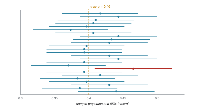
Common misreadings are worth naming. A 95 percent confidence interval does not mean that 95 percent of the individuals fall in the interval; it is about a parameter, such as a mean, not about individual values. It does not mean there is a 95 percent probability that this particular interval contains the parameter in the sense of a coin not yet tossed; the parameter is fixed and the interval either contains it or not. And it says nothing about bias: if the sample was badly chosen, the interval can be confidently wrong.
A confidence interval for a proportion
For a population proportion p, the estimate is the sample proportion \(\hat{p}\), and its standard error is \(SE = \sqrt{\hat{p}(1 - \hat{p})/n}\). The 95 percent confidence interval is \(\hat{p} \pm 1.96\,SE\). The critical value 1.96 comes from the standard normal distribution: 95 percent of the area lies between -1.96 and 1.96. For other confidence levels use 1.645 for 90 percent and 2.576 for 99 percent.
The interval is reliable when the sample is a random sample from a population at least ten times larger and when there are at least 10 successes and 10 failures in the sample. With smaller counts, an adjusted method, such as adding two successes and two failures before computing (sometimes called the plus-four method), works much better.
# 95% confidence interval for a proportion: 248 of 400 residents support a new bus route.
import math
from statistics import NormalDist
x, n = 248, 400
phat = x / n
se = math.sqrt(phat * (1 - phat) / n)
for level in (0.90, 0.95, 0.99):
    z = NormalDist().inv_cdf(1 - (1 - level) / 2)
print(f"{level:.0%} CI: {phat:.3f} +/- {z:.3f} x {se:.4f} = ({phat - z * se:.3f}, {phat + z * se:.3f})")90% CI: 0.620 +/- 1.645 x 0.0243 = (0.580, 0.660) 95% CI: 0.620 +/- 1.960 x 0.0243 = (0.572, 0.668) 99% CI: 0.620 +/- 2.576 x 0.0243 = (0.557, 0.683)
In context: we are 95 percent confident that between about 57 and 67 percent of all residents support the new route. Note the trade-off between confidence and precision: a 99 percent interval is wider than a 95 percent one, which is wider than a 90 percent one. You cannot have high confidence and a narrow interval without collecting more data.
Polls and the margin of error
For a poll, the margin of error is the plus-or-minus part of the interval. Pollsters usually report the margin for a sample proportion of 0.5, because that gives the largest possible margin for a given sample size: \(1.96\sqrt{0.5 \times 0.5/n} \approx 1/\sqrt{n}\). That is why a poll of about 1,000 people reports a margin of error of about plus or minus 3 percentage points, 19 times out of 20, and a poll of about 2,500 reports about 2 points.
| Sample size n | Approximate 95% margin of error (p near 0.5) |
|---|---|
| 100 | ± 9.8 percentage points |
| 400 | ± 4.9 points |
| 1,000 | ± 3.1 points |
| 1,500 | ± 2.5 points |
| 2,500 | ± 2.0 points |
| 10,000 | ± 1.0 point |
Two cautions apply. The margin of error for a subgroup, such as young adults or one province or state, is much larger than for the whole sample, because the subgroup sample is smaller. And the margin of error covers only random sampling variability. It does not cover non-response bias, coverage problems, question wording or last-minute changes of opinion, which is why polls sometimes miss by more than their stated margin. Many online panels are not random samples at all; reputable pollsters that use them describe their results with a credibility interval or similar term and explain their weighting.
A confidence interval for a mean
For a population mean \(\mu\), the estimate is the sample mean \(\bar{x}\), and its standard error is \(SE = s/\sqrt{n}\), using the sample standard deviation s because we do not know the population standard deviation \(\sigma\). Replacing \(\sigma\) with s adds extra uncertainty, especially in small samples. To account for it, we use a critical value from the t distribution instead of the normal distribution.
The t distributions, discovered by William Gosset while working on quality control at the Guinness brewery in Dublin in the early 1900s, look like the standard normal curve but with heavier tails. There is a different t distribution for each sample size, identified by its degrees of freedom, df = n - 1. With few degrees of freedom the tails are much heavier and the critical values larger; as n grows, the t distribution approaches the standard normal. For df = 9 the 95 percent critical value is 2.262; for df = 29 it is 2.045; for df = 99 it is 1.984, already close to 1.96.
The one-sample t interval is \(\bar{x} \pm t^*\,\frac{s}{\sqrt{n}}\), where \(t^*\) is the critical value with n - 1 degrees of freedom. It requires a random sample and a population distribution that is roughly normal, or a large enough sample for the central limit theorem to apply. In practice: for n under 15, use it only if the data look close to normal with no outliers; for n of 15 to 40, it is fine unless there are outliers or strong skewness; for n over 40, it works well even for skewed data.
# One-sample t interval for the mean commute time (invented random sample of 400 residents).
import random, statistics as st, math
from scipy import stats            # scipy.stats provides t-distribution critical values
random.seed(141)
times = [random.gammavariate(3.2, 7.7) for _ in range(400)]
n, xbar, s = len(times), st.mean(times), st.stdev(times)
se = s / math.sqrt(n)
tstar = stats.t.ppf(0.975, df=n - 1)
print(f"n = {n}, sample mean = {xbar:.2f} min, s = {s:.2f} min, SE = {se:.3f}")
print(f"t* (df = {n - 1}) = {tstar:.3f}")
print(f"95% CI for the mean commute: ({xbar - tstar * se:.2f}, {xbar + tstar * se:.2f}) minutes")
# A small sample of 12 gives a much wider interval
small = times[:12]
t12 = stats.t.ppf(0.975, df=11)
m12, se12 = st.mean(small), st.stdev(small) / math.sqrt(12)
print(f"with only 12 residents: t* = {t12:.3f}, 95% CI = ({m12 - t12 * se12:.1f}, {m12 + t12 * se12:.1f}) minutes")n = 400, sample mean = 25.13 min, s = 13.93 min, SE = 0.696 t* (df = 399) = 1.966 95% CI for the mean commute: (23.76, 26.50) minutes with only 12 residents: t* = 2.201, 95% CI = (17.3, 31.0) minutes
The survey of 400 pins down the mean commute to within about one and a half minutes either way. The same calculation with only 12 residents gives an interval several times as wide, both because the standard error is larger and because the critical value is larger. Note that commute times are skewed to the right, but with 400 observations the central limit theorem makes the interval trustworthy; with 12, the skewness would be a real concern.
Choosing a sample size
Before collecting data, you can decide how large a sample you need to achieve a desired margin of error. For a proportion, solving \(m = z^*\sqrt{p(1-p)/n}\) for n gives \(n = \left(\frac{z^*}{m}\right)^2 p(1 - p)\). If you have no idea what p is, use 0.5, which gives the largest, safest answer. For a mean, \(n = \left(\frac{z^* \sigma}{m}\right)^2\), using an estimate of \(\sigma\) from a pilot study or earlier research. Always round up.
# Sample size needed for a desired margin of error (95% confidence).
import math
z = 1.96
for m in (0.05, 0.03, 0.02, 0.01):
    n = math.ceil((z / m) ** 2 * 0.25)
    print(f"proportion, margin +/- {m:.0%}: n = {n:,}")
sigma = 15          # minutes, rough SD of commute times from a pilot
for m in (3, 2, 1):
print(f"mean commute, margin +/- {m} min: n = {math.ceil((z * sigma / m) ** 2):,}")proportion, margin +/- 5%: n = 385 proportion, margin +/- 3%: n = 1,068 proportion, margin +/- 2%: n = 2,401 proportion, margin +/- 1%: n = 9,604 mean commute, margin +/- 3 min: n = 97 mean commute, margin +/- 2 min: n = 217 mean commute, margin +/- 1 min: n = 865
The square-root law from lesson 9 appears again: each halving of the margin of error roughly quadruples the sample size and, with it, the cost. A city planning a transit survey might reasonably settle for a margin of plus or minus 5 percentage points with about 400 respondents rather than plus or minus 1 point with nearly 10,000.
Worked problem
Building and interpreting a confidence interval
Aisha takes a random sample of 64 clinic visits and records the time from check-in to seeing a nurse. The sample mean is 18.4 minutes and the standard deviation is 9.6 minutes. Construct and interpret a 95 percent confidence interval for the mean time, given t* = 1.998 for 63 degrees of freedom. Would a 99 percent interval be wider or narrower?
Show solution
- Conditions: a random sample of visits; n = 64 is large enough for the central limit theorem even if times are skewed.
- Standard error: 9.6 / sqrt(64) = 9.6 / 8 = 1.2 minutes.
- Margin of error: 1.998 x 1.2 = 2.40 minutes.
- Interval: 18.4 ± 2.40, or about 16.0 to 20.8 minutes.
- Interpretation: we are 95 percent confident that the mean time to see a nurse for all clinic visits is between about 16.0 and 20.8 minutes.
- A 99 percent interval would use a larger critical value, so it would be wider.
Answer: About 16.0 to 20.8 minutes with 95 percent confidence; a 99 percent interval would be wider.
Common mistakes
MistakeSaying that 95 percent of individuals fall inside the confidence interval.
InsteadThe interval estimates a parameter such as the mean, not the range of individual values.
MistakeSaying there is a 95 percent chance this particular interval contains the parameter.
InsteadThe 95 percent describes how often the method succeeds over many samples.
MistakeAssuming the margin of error covers bias from non-response or poor wording.
InsteadIt covers random sampling variability only.
MistakeUsing the normal critical value 1.96 for a mean from a small sample.
InsteadUse a t critical value with n - 1 degrees of freedom.
MistakeReporting a subgroup result with the whole sample's margin of error.
InsteadSubgroups are smaller and have larger margins of error.
Summary and key terms
- A confidence interval has the form estimate plus or minus margin of error, where the margin is a critical value times the standard error.
- The confidence level describes how often the method captures the parameter over many samples.
- For a proportion: p hat ± z* sqrt(p hat (1 - p hat)/n), with at least 10 successes and 10 failures.
- A poll of about 1,000 has a margin of error near ± 3 points; subgroups and non-sampling errors add uncertainty.
- For a mean: x bar ± t* s/sqrt(n) with n - 1 degrees of freedom; t critical values exceed z values in small samples.
- Required sample size grows with the square of the desired precision: halving the margin needs about four times as much data.
- confidence interval
- An interval of plausible values for a parameter, calculated from sample data by a method with a known success rate.
- confidence level
- The proportion of samples for which the method produces an interval containing the parameter.
- margin of error
- The plus-or-minus part of a confidence interval.
- critical value
- The multiplier of the standard error that sets the confidence level, such as 1.96 for 95 percent.
- standard error
- The estimated standard deviation of a statistic.
- t distribution
- A family of bell-shaped distributions with heavier tails than the normal, used for means when sigma is estimated.
- degrees of freedom
- The parameter of a t distribution, n - 1 for a one-sample mean.
Practice problems
Work each problem on paper first, then reveal the answer to check.
In a sample of 500, 210 say yes. Find p hat and its standard error.
Show answer
p hat = 0.42; SE = sqrt(0.42 x 0.58 / 500) = 0.0221.
Find the 95 percent confidence interval for the previous question.
Show answer
0.42 ± 0.043, about 0.377 to 0.463.
A poll reports 46 percent with a margin of ± 3 points. Could the true support be 50 percent?
Show answer
It is just outside the interval (43 to 49 percent), so 50 percent is not among the plausible values, though non-sampling errors add uncertainty.
Approximately what margin of error does a poll of 2,500 have?
Show answer
About ± 2 percentage points.
Why is t* larger than 1.96 for small samples?
Show answer
Estimating sigma with s adds uncertainty, so the t distribution has heavier tails.
How large a sample gives a margin of ± 4 points for a proportion (95 percent, p unknown)?
Show answer
(1.96 / 0.04)^2 x 0.25 = 600.25, so 601.
A 95 percent interval for a mean is 40 to 50. What is the sample mean and the margin of error?
Show answer
Mean 45, margin 5.
What happens to a confidence interval if the confidence level is raised from 95 to 99 percent?
Show answer
It becomes wider.
Lesson quiz · 5 questions
Score 60% or more to complete this lesson.
Create a free account to save your progress, take quizzes and earn a certificate.