
NUC-350 · Lesson 10 of 12 · 20 min
Monte Carlo methods
A question comes in from the station: a new type of flux detector assembly is to be installed between two channels, and the shutdown systems group wants to know how it changes the worth of the nearest shutoff rod. "Our diffusion model cannot see that level of detail," Teodora says. "We will build a Monte Carlo model of a small region of the core, every bundle and tube, and compare. Monte Carlo is how we check the deterministic codes when the geometry gets complicated."
The idea of Monte Carlo transport
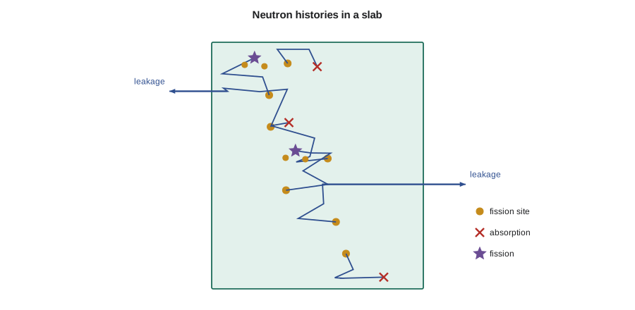
Deterministic methods such as diffusion theory, discrete ordinates or the method of characteristics solve equations for the average behaviour of neutrons on a mesh of space, energy and angle. The Monte Carlo method instead simulates the life histories of individual neutrons, one at a time, using random numbers to sample each event from the physical probability laws. A neutron is born at a fission site with an energy sampled from the fission spectrum and a direction sampled at random. It travels a distance sampled from the exponential law of free flight, collides with a nucleus chosen in proportion to its cross section, and either scatters to a new energy and direction, is captured or causes fission. The history continues until the neutron is absorbed or leaks. Averages over many histories estimate any quantity of interest: k, fluxes, reaction rates or doses.
The distance to the next collision is sampled from the probability density Σ_t e^{−Σ_t s}. Using a random number ξ uniformly distributed between zero and one, the sampled distance is:
Each type of event is sampled in the same way, from its own probability law. The method's great strength is that it can represent geometry and energy almost exactly. The geometry can be described by combinations of surfaces, cylinders, planes and spheres, so that every pin, gap and tube is modelled as it is. Cross sections can be used in continuous energy, directly from evaluated nuclear data, without any group structure or self-shielding approximation. Monte Carlo codes are therefore the reference against which lattice and core methods are tested.
Estimating k by generations
For a critical or near-critical system, the eigenvalue k is estimated by following neutrons in generations. A batch of N neutrons is started from a guessed distribution of fission sites. Each neutron is followed until it is absorbed or leaks, and every fission records new sites with a number of neutrons sampled from ν. The ratio of the number of new fission neutrons to N estimates k for that generation. The new fission sites become the source for the next generation, renormalized to N neutrons. After enough inactive generations for the source shape to converge, further active generations are averaged to estimate k and its statistical uncertainty.
The program below follows one-speed neutrons with isotropic scattering in a homogeneous slab 60 cm thick, with reactor-like macroscopic cross sections. It runs 30 generations of 4 000 neutrons, discards the first eight as inactive and compares the Monte Carlo k with the one-group diffusion result for the same slab.
# Monte Carlo: one-speed neutrons in a homogeneous slab of reactor-like material.
# Each generation starts from fission sites of the last; k is the ratio of new
# fission neutrons to starting neutrons. Compared with one-group diffusion theory.
import math, random
rng = random.Random(2026)
St, Sa, nSf = 0.40, 0.030, 0.033     # 1/cm (illustrative homogenized values)
Ss = St - Sa
width = 60.0                          # slab thickness, cm (infinite in y and z)
def generation(sites):
    new = []
    for x in sites:
        mu = 2 * rng.random() - 1
        while True:
            x += mu * (-math.log(rng.random()) / St)
            if x < 0 or x > width: break                   # leaked
            if rng.random() < Sa / St:                     # absorbed
                nu_expected = nSf / Sa
                for _ in range(int(nu_expected + rng.random())): new.append(x)
                break
            mu = 2 * rng.random() - 1                      # isotropic scatter
    return new
N = 4000
sites = [rng.uniform(0, width) for _ in range(N)]
ks = []
for g in range(30):
    new = generation(sites)
    ks.append(len(new) / len(sites))
    sites = [rng.choice(new) for _ in range(N)]          # renormalize population
active = ks[8:]
mean = sum(active) / len(active)
sd = math.sqrt(sum((k - mean) ** 2 for k in active) / (len(active) - 1) / len(active))
print(f"Monte Carlo k = {mean:.4f} +/- {sd:.4f} (from {len(active)} active generations of {N} neutrons)")
D = 1 / (3 * St); L2 = D / Sa; d = 0.71 / St
B2 = (math.pi / (width + 2 * d)) ** 2
print(f"one-group diffusion k = {nSf / Sa / (1 + L2 * B2):.4f} (k_inf = {nSf / Sa:.3f}, L = {math.sqrt(L2):.2f} cm)")Monte Carlo k = 1.0316 +/- 0.0013 (from 22 active generations of 4000 neutrons) one-group diffusion k = 1.0301 (k_inf = 1.100, L = 5.27 cm)
The two methods agree to within about two standard deviations of the Monte Carlo estimate. That is to be expected here: the slab is many mean free paths thick and the material is homogeneous, so diffusion theory is accurate. In a heterogeneous lattice, near strong absorbers or close to boundaries, the two would differ more, and the Monte Carlo result, being free of the diffusion approximation, would be the more trustworthy. That is precisely the role Monte Carlo plays in practice.
Statistics and uncertainty
A Monte Carlo result is an estimate with a statistical uncertainty. If each active generation gives an estimate k_i, the mean and its standard error are:
The standard error falls in proportion to the inverse square root of the number of histories. Halving the uncertainty therefore needs four times as many histories. For k, uncertainties of 10 pcm or less are routine with modern computers. For local quantities such as the power in one pin or the flux in a small detector, many more histories are needed, because only a small fraction of neutrons contribute to each tally.
Worked problem
How many histories?
A calculation with 10 million histories gives a pin power with a relative standard error of 1.2 percent. How many histories are needed to reach 0.3 percent?
Show solution
- The error scales as 1/√N, so N scales as the square of the error ratio.
- (1.2/0.3)² = 16.
- 16 × 10 million = 160 million histories.
Answer: Reaching four times better precision costs sixteen times more computing, which is why variance reduction and careful tally design matter in practice.
Pitfalls in eigenvalue calculations
Two problems need care. The first is source convergence. In a large, loosely coupled core with a dominance ratio close to one, the fission source shape converges slowly, just as it does in the deterministic power iteration of lesson 1. If active generations begin too early, the results are biased toward the initial guess. Diagnostics such as the Shannon entropy of the source distribution show when the source has settled. The second problem is correlation between generations: because each generation's source comes from the previous one, successive k estimates are not independent, and the simple formula above can underestimate the true uncertainty of local tallies. Codes and analysts allow for this by using enough neutrons per generation and by batching generations.
Variance reduction
When the quantity of interest is in a region that few neutrons reach, such as a detector far from the core or a dose point behind a shield, analog Monte Carlo is inefficient. Variance reduction methods change the sampling so that more neutrons go where they are needed while each carries a statistical weight that keeps the estimate unbiased. Implicit capture lets a neutron survive every collision with a reduced weight instead of being absorbed. Russian roulette ends low-weight histories with a probability that preserves the expected weight. Splitting divides a neutron into several of lower weight as it moves toward an important region. Weight windows, often generated automatically from a deterministic adjoint calculation, combine these ideas. Shielding problems for vessels and spent fuel casks rely heavily on such methods.
Monte Carlo codes in practice
In the Canadian industry, Monte Carlo codes are used to validate lattice and core methods and for special studies such as detector responses, device worths and criticality safety. Codes include MCNP, developed at Los Alamos, SERPENT, developed in Finland and widely used in research, and OpenMC, an open-source code developed by a community led by U.S. national laboratories. Canadian Nuclear Laboratories and universities have also developed and used Monte Carlo methods for CANDU lattices, where the complex cluster geometry suits continuous-energy Monte Carlo especially well. Licensing calculations for operating cores still rely mainly on deterministic codes, validated against Monte Carlo and measurements.
Monte Carlo methods are also moving into routine core analysis. With large computing clusters, full-core Monte Carlo calculations with pin-level detail and depletion are now possible for research and benchmark purposes. Such calculations are coupled with thermal hydraulic codes to include temperature feedback. They remain too expensive for the thousands of cases needed in each reload design, but they provide reference solutions against which faster methods are measured, and they are increasingly used to generate lattice constants directly.
Benchmarks and validation
Whether deterministic or Monte Carlo, every code must be validated against measured data. Critical experiments, in which small assemblies of fuel are brought to criticality under carefully controlled conditions, provide the most direct test of k. International benchmark collections, built up over decades by the OECD Nuclear Energy Agency and its member countries, document hundreds of such experiments with uncertainties. Code developers and users calculate these benchmarks to show that a code with a given nuclear data library predicts k within a known bias and uncertainty. Power reactor measurements, such as critical boron, rod worths and in-core detector readings, provide further validation for the complete calculation chain.
Monte Carlo for depletion and criticality safety
Monte Carlo codes can also deplete fuel. In a Monte Carlo depletion calculation, each step consists of a transport calculation that tallies reaction rates in every fuel region, followed by a solution of the Bateman equations of lesson 4 for those regions. Because the transport calculation has statistical noise, the depleted compositions carry that noise forward, and the step lengths and numbers of histories must be chosen with care. Such calculations are used to produce reference results for lattice codes and to study fuel designs that deterministic codes model less well.
Criticality safety is another major use. Outside the reactor, fresh and spent fuel must be kept well subcritical in storage racks, transport casks and fuel handling, under normal and accident conditions such as flooding or misloading. Regulators in Canada and the United States require that the calculated k of such systems, including biases and uncertainties, stays below an upper limit, commonly 0.95 for many storage applications. Monte Carlo codes, validated against critical experiments, are the standard tool for these analyses because they can model complex rack and cask geometries exactly.
| Application | What Monte Carlo provides | Why it is preferred |
|---|---|---|
| Lattice code validation | reference k and pin powers | continuous energy and exact geometry |
| Device and detector studies | local reaction rates and worths | complex geometry near the device |
| Criticality safety of storage and transport | k with uncertainty for racks and casks | exact geometry and validated data |
| Shielding and vessel fluence | deep-penetration fluxes with variance reduction | handles streaming and complex paths |
Random numbers deserve a final word. Monte Carlo codes use pseudo-random number generators, deterministic algorithms that produce long sequences with good statistical properties. A given starting seed always gives the same sequence, which allows calculations to be repeated exactly for quality assurance. The generators are tested to make sure that their sequences are long enough and free of correlations that could bias results, and parallel calculations give each processor its own well-separated part of the sequence.
Teodora's detector study shows the method at work. The Monte Carlo model of the region around the new assembly gives the change in local worth with an uncertainty of a few percent, enough to confirm that the effect is small. The comparison with the deterministic model, which treats the assembly in a simplified way, shows a difference within the expected range, so the deterministic model can still be used for routine calculations with a small, documented correction.
Common mistakes
MistakeA Monte Carlo result is exact because it uses the real geometry.
InsteadIt is an estimate with a statistical uncertainty, and it also depends on the nuclear data used.
MistakeDoubling the number of histories halves the uncertainty.
InsteadThe uncertainty falls as the inverse square root of histories; four times as many are needed to halve it.
MistakeEvery generation in an eigenvalue calculation can be counted.
InsteadEarly inactive generations must be discarded until the fission source shape has converged.
Summary and key terms
- Monte Carlo methods simulate individual neutron histories with random sampling of physical events.
- They can model geometry and energy almost exactly and serve as reference solutions.
- k is estimated by generations, discarding inactive ones until the source converges.
- Statistical uncertainty falls as one over the square root of the number of histories.
- Variance reduction methods make deep-penetration and small-region problems feasible.
- History
- The simulated life of one neutron from birth to absorption or leakage.
- Tally
- A quantity accumulated during a Monte Carlo calculation, such as a flux or reaction rate.
- Inactive generation
- An early generation discarded while the fission source converges.
- Standard error
- The statistical uncertainty of a Monte Carlo mean.
- Variance reduction
- Sampling changes that reduce uncertainty for a given computing effort without biasing the result.
- Shannon entropy
- A measure of the spread of the fission source used to judge its convergence.
Practice problems
Work each problem on paper first, then reveal the answer to check.
How is the distance to the next collision sampled?
Show answer
s = −ln(ξ)/Σ_t, with ξ a uniform random number.
Why are inactive generations discarded?
Show answer
The fission source distribution must converge before k and tallies are averaged.
In the example, how many histories give 0.3 percent?
Show answer
About 160 million.
Name two variance reduction techniques.
Show answer
Implicit capture and Russian roulette; splitting and weight windows are others.
Why are deterministic codes still used for reload licensing?
Show answer
Monte Carlo is too expensive for the thousands of cases needed; deterministic codes are validated against it.
Lesson quiz · 5 questions
Score 60% or more to complete this lesson.
Create a free account to save your progress, take quizzes and earn a certificate.