
MSAZ-319 · Lesson 7 of 12 · 20 min
Reading DAX, SQL and PySpark in questions
▶ Video coming soon A video version of this lesson is on the way.
Many DP-600 items show a block of code and ask what it returns, which line is wrong, or which keyword completes it. The candidate does not run anything; the skill is reading. On Monday, November 30, Marisol gave Keiko a stack of short listings in four languages, DAX, T-SQL, PySpark and KQL, and asked her to say in one sentence what each did before looking at any options. Keiko writes DAX and T-SQL every week, reads PySpark a few times a month and had written only three KQL queries, so the evening showed clearly where her reading was slow.
This lesson works through one listing in each language, then gives a method for reading code under time pressure. The listings are short on purpose: exam items rarely show more than fifteen lines, and the hard part is usually one keyword, one filter or one join type.
A method for reading code in an item
Marisol's method has four steps. First, find the output: in DAX, the RETURN expression or the measure's result; in SQL, the SELECT list; in PySpark, the last write or display; in KQL, the last operator. Second, find the source and the filters: which table, which WHERE, filter or where clause, and which joins. Third, find the grouping: GROUP BY, groupBy, summarize by, or the filter context in DAX. Fourth, look for the one detail the item is about, which is usually a join type, a null, a date boundary or a filter that applies at the wrong step. Saying the result in plain words before reading the options stops a plausible option from deciding for you.
| Language | Output | Source and filters | Grouping | Common trap |
|---|---|---|---|---|
| DAX | RETURN or measure result | CALCULATE filters, FILTER | Filter context of the visual | ALL removing a filter the item needs |
| T-SQL | SELECT list | FROM, JOIN, WHERE | GROUP BY, HAVING | INNER JOIN dropping unmatched rows |
| PySpark | write, saveAsTable, display | read, filter, join | groupBy, agg | Overwrite where append was meant |
| KQL | Last operator | Table, where | summarize by | bin size or ago() window |
DAX
DAX items usually turn on filter context. The measure below counts the stores that sold more than a target in the selected period.
Stores Above Target =
VAR Target = 250000
RETURN
    COUNTROWS (
        FILTER (
            VALUES ( 'Store'[Store Key] ),
            [Net Sales] > Target
        )
    )
Read it with the method. The output is a count of rows. The source is the list of store keys visible in the current filter context, from VALUES. The filter keeps only stores whose net sales exceed 250,000; because [Net Sales] is a measure, it is evaluated for each store by context transition. The grouping is whatever the visual groups by: on a card with no other filters it counts across all stores; in a table by region it counts within each region. An item might ask what changes if VALUES is replaced by ALL('Store'[Store Key]); the answer is that the count would ignore filters on the store table, such as a region slicer, which is usually wrong.
T-SQL
SQL items often test joins and nulls. The query below lists stores and their sales for November 2026.
SELECT s.store_name,
       SUM(f.net_amount) AS net_sales
FROM dbo.dim_store AS s
LEFT JOIN dbo.fact_sales AS f
       ON f.store_key = s.store_key
WHERE f.sale_date >= '2026-11-01'
  AND f.sale_date <  '2026-12-01'
GROUP BY s.store_name;
The output is one row per store with its net sales. The join is a LEFT JOIN, which suggests that stores without sales should appear with a null total. But the WHERE clause filters on columns of fact_sales, and for a store with no sales those columns are null, so the WHERE removes it. The LEFT JOIN behaves like an INNER JOIN. To keep stores without sales, the date conditions move into the ON clause. This is one of the most common SQL traps on the exam, and Keiko missed it on the diagnostic.
PySpark
PySpark items usually show a short transformation in a notebook. The listing below cleans the day's sales lines and adds them to a lakehouse table.
df = spark.read.table("lh_raw.sales_lines")
clean = (df.filter(df.quantity > 0)
           .dropDuplicates(["receipt_id", "line_no"])
           .withColumn("net_amount", df.unit_price * df.quantity - df.discount_amt))
clean.write.mode("append").format("delta").saveAsTable("lh_clean.sales_lines")
The output is an append to the Delta table lh_clean.sales_lines. The source is lh_raw.sales_lines, filtered to positive quantities, which removes returns. Duplicates are removed on the receipt and line number. The new column computes the net amount. An item could ask what happens if the cell runs twice for the same day: because the mode is append and nothing checks for rows already loaded, the day's lines are added twice. The fixes are a MERGE on the key, or overwriting only the day's partition. Another item could ask why returns disappear from the clean table, which is the quantity filter.
KQL
KQL items appear in questions about eventhouses and real-time data. The query below looks for tills that have stopped sending events.
TillEvents
| where Timestamp > ago(30m)
| summarize LastEvent = max(Timestamp) by StoreId, TillId
| where LastEvent < ago(10m)
| project StoreId, TillId, LastEvent
| order by LastEvent asc
The output is a list of stores and tills with their last event time, oldest first. The source is events from the last 30 minutes. The grouping is by store and till, keeping the latest timestamp. The second where keeps tills whose latest event is more than ten minutes old. The trap is the first filter: a till that has been silent for more than 30 minutes has no events in the window, so it does not appear at all. An item might ask how to include it, and the answer is to compare against a list of all tills rather than only the tills that sent events.
Seeing the join trap with real rows
Keiko understood the LEFT JOIN trap once she saw it with a handful of rows. Marisol wrote the short listing below, which joins three stores to four sales lines in plain Python, first with the date filter applied after the join, as a WHERE clause would, then with the filter applied inside the join, as an ON clause would. It runs in the browser.
stores = ["Store 101", "Store 102", "Store 103"]
sales = [("Store 101", "2026-11-03", 1200), ("Store 101", "2026-10-28", 800),
         ("Store 102", "2026-11-12", 950), ("Store 103", "2026-10-15", 400)]

def in_november(day):
    return "2026-11-01" <= day < "2026-12-01"

# Filter after the join, like WHERE
after = {}
for store in stores:
    matches = [s for s in sales if s[0] == store] or [(store, None, None)]
    for _, day, amount in matches:
        if day is not None and in_november(day):
            after[store] = after.get(store, 0) + amount
print("Filter in WHERE:", after)

# Filter inside the join, like ON
inside = {}
for store in stores:
    matches = [s for s in sales if s[0] == store and in_november(s[1])]
    inside[store] = sum(m[2] for m in matches) if matches else None
print("Filter in ON: ", inside)Filter in WHERE: {'Store 101': 1200, 'Store 102': 950}
Filter in ON: {'Store 101': 1200, 'Store 102': 950, 'Store 103': None}What this code does
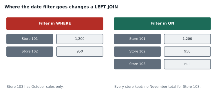
The listing sets up three stores and four sales lines, one of them for Store 103 in October only. The first loop joins each store to its sales and keeps a row only if its date is in November, which is what a WHERE clause does after a left join, so Store 103 disappears. The second loop applies the November test while matching, which is what an ON clause does, so Store 103 stays in the result with no total.
The first result has two stores; the second has all three, with Store 103's total empty. That is exactly the difference between the two versions of the SQL query in the lesson. The same pattern appears in DAX when a filter is applied to the fact table instead of through the dimension, and in PySpark when a filter on the right-hand table follows a left join instead of preceding it.
Power Query M
Although M is not named in the outline as often as the other languages, dataflow items sometimes show a few steps of a query. Each step is a line in a let expression that refers to the previous one by name, and the last name after in is the output.
let
    Source = Csv.Document(File.Contents("supplier_prices.csv"), [Delimiter = ","]),
    Promoted = Table.PromoteHeaders(Source),
    Typed = Table.TransformColumnTypes(Promoted, {{"unit_cost", type number}, {"effective_date", type date}}),
    Current = Table.SelectRows(Typed, each [effective_date] <= Date.From(DateTime.LocalNow()))
in
    Current
Read it with the same method. The output is the step called Current. The source is a CSV file of supplier prices with headers promoted. The types are set before the filter, which matters: comparing text to a date would fail or behave unexpectedly. The filter keeps prices effective up to today. An item might ask why the query does not fold to the source, and for a CSV file the answer is that files cannot fold at all; folding applies to sources such as databases.
DAX windowing functions
The newer windowing functions, WINDOW, OFFSET and INDEX, appear in the outline and in items that ask for a running total or a comparison with the previous row. OFFSET(-1, ...) returns the previous row in a given order, so a measure that subtracts the previous month's sales from the current month's can be written without date intelligence functions. WINDOW returns a range of rows, such as the three months up to the current one for a rolling average. Each takes an ORDERBY and, optionally, a PARTITIONBY that restarts the order within each group, such as each store. Keiko had not used them before; she found it easiest to think of them as SQL window functions written in DAX, with ORDERBY and PARTITIONBY playing the same roles as ORDER BY and PARTITION BY in an OVER clause.
| DAX | Closest T-SQL | Typical use |
|---|---|---|
| OFFSET(-1, ...) | LAG() | Change from the previous month |
| WINDOW(-2, REL, 0, REL, ...) | AVG() OVER (ROWS BETWEEN 2 PRECEDING AND CURRENT ROW) | Three-month rolling average |
| INDEX(1, ...) | FIRST_VALUE() | First month in the period |
| RANKX | RANK() | Ranking stores by sales |
Reading a windowing function in an item comes down to three questions: which rows are ordered, in which order, and where the order restarts. A missing PARTITIONBY is the usual mistake: without it, a running total by store runs across all stores instead of restarting for each one. Keiko now checks for PARTITIONBY first whenever an item shows a windowing function grouped by store or region, and she adds a line to her error log every time she misses it in practice, so that by the September timed sets the habit is automatic.
Worked problem
Saying a listing in one sentence
Summarize the KQL query above in one sentence before reading any options, then name one case it misses.
Show solution
- Output: stores and tills with their last event, oldest first.
- Source and filter: events in the last 30 minutes.
- Grouping: by store and till, latest timestamp.
- Second filter: latest event more than ten minutes ago.
- Missed case: tills silent for more than 30 minutes, which have no events in the window.
Answer: It lists tills that sent events in the last half hour but none in the last ten minutes; tills silent for longer than half an hour are missed.
Common mistakes
MistakeAssume a LEFT JOIN always keeps unmatched rows.
InsteadA WHERE filter on the right table's columns removes them; move the filter into ON.
MistakeReplace VALUES with ALL without thinking about slicers.
InsteadALL ignores filters on the column, so slicers stop affecting the count.
MistakeAppend mode is safe to rerun.
InsteadRerunning an append duplicates the rows; use MERGE or overwrite a partition.
MistakeA KQL summarize finds missing items.
InsteadIt can only group rows that exist; compare against a full list to find what is missing.
MistakeRead options before the code.
InsteadSay what the code does first, then read the options.
Summary and key terms
- Read code in four steps: output, source and filters, grouping, then the one detail the item is about.
- DAX items turn on filter context, context transition and functions such as VALUES and ALL.
- SQL items often test join types, where filters sit, and nulls.
- PySpark items test filters, deduplication, write modes and what happens on rerun.
- KQL items test where, summarize by, bin() and the time window chosen with ago().
- Say the result in plain words before reading the options.
- Context transition
- DAX turning the current row of an iterator into a filter when a measure is evaluated inside it.
- LEFT JOIN
- A join that keeps every row from the left table, with nulls where the right table has no match.
- Write mode
- The option that decides whether a Spark write appends, overwrites or fails when the table exists.
- summarize
- The KQL operator that aggregates rows, grouped by the columns after by.
- ago()
- A KQL function that returns a time a given interval before now.
Practice problems
Work each problem on paper first, then reveal the answer to check.
In the T-SQL query, why do stores with no November sales disappear?
Show answer
The WHERE filter on fact_sales columns removes rows where those columns are null.
What happens if the PySpark cell runs twice for the same day?
Show answer
The day's lines are appended twice.
In the DAX measure, what does VALUES('Store'[Store Key]) return?
Show answer
The store keys visible in the current filter context.
Which tills does the KQL query miss?
Show answer
Tills silent for more than 30 minutes.
What is the first step of the reading method?
Show answer
Find the output.
Lesson quiz · 5 questions
Score 60% or more to complete this lesson.
Create a free account to save your progress, take quizzes and earn a certificate.