
MSAZ-319 · Lesson 5 of 12 · 21 min
Review: preparing data
▶ Video coming soon A video version of this lesson is on the way.
Preparing data is the largest area on the current outline, almost half of the exam by the most often quoted estimate, and Keiko's weakest at 11 of 20 on the diagnostic. It is also the broadest. It covers getting data into a lakehouse, warehouse or eventhouse, creating the objects that hold and expose it, transforming it into a shape the semantic model can use, querying it, and fixing performance problems on the way. Marisol split the review into two evenings, Monday and Tuesday, November 23 and 24, and this lesson follows the same order: get data, transform data, query and analyze data, and optimize.
The fall courses gave Keiko most of the raw material. The supplier price files arrived through a dataflow; the sales lines were cleaned in a notebook; the star schema was built in wh_sales with T-SQL; and the model read it through Direct Lake. What the diagnostic showed is that she knew the path she had built better than the alternatives, and exam items are almost always about choosing among alternatives.
Get data: connections, stores and shortcuts
The first decision is where the data should live. A lakehouse stores data as files and Delta tables in OneLake and is the natural home for data loaded and transformed with Spark or dataflows; it has a read-only SQL analytics endpoint for querying tables with T-SQL. A warehouse is a full T-SQL environment with read-write tables, transactions across tables, views, functions and stored procedures; it suits teams that work in SQL and need write access through SQL. An eventhouse holds KQL databases for streaming and time-series data that must be queried within seconds of arrival. All three store their data in OneLake in open formats, so one engine can often read what another wrote.
Shortcuts let a lakehouse or KQL database point at data stored elsewhere without copying it: in another Fabric item, in Azure Data Lake Storage, in Amazon S3, in Google Cloud Storage or in other supported locations. A shortcut appears as a folder or table and can be read by every engine that reads the lakehouse. The rules are worth knowing: access goes through the shortcut's connection or the user's identity depending on the target, the security of the target still applies, and deleting a shortcut does not delete the data it points to. Mirroring is the other way to bring data in without building pipelines: it keeps a near-real-time copy of an operational database, such as Azure SQL Database or Snowflake, in OneLake as Delta tables.
| Need | Best fit | Why not the others |
|---|---|---|
| Data already in another Fabric lakehouse, read by Spark and SQL | Shortcut | Copying wastes storage and goes stale |
| Near-real-time copy of an operational database without code | Mirroring | A pipeline needs scheduling and change logic |
| Low-code transformation from many file types by analysts | Dataflow Gen2 | A notebook needs Spark skills |
| Large, complex transformation in Python or Spark SQL | Notebook | A dataflow becomes slow and hard to test |
| Transformation by a team that works in SQL, writing to the warehouse | T-SQL in the warehouse (stored procedures, CTAS) | The lakehouse endpoint is read-only |
| Streaming events queried within seconds | Eventstream into an eventhouse | Batch loads are too slow |
Ingesting and copying
For moving data into Fabric, the outline names data pipelines, dataflows and notebooks, and the choice is mostly about skills and volume. A data pipeline's Copy activity, or a copy job, moves data from a source to a lakehouse or warehouse with little transformation, at scale, on a schedule or a trigger. A Dataflow Gen2 uses Power Query, the same tool as in Power BI Desktop, to connect, clean and write to a destination, which suits analysts and moderate volumes. A notebook uses Spark and suits large volumes and logic that is easier in code. A pipeline can also orchestrate the others: run a dataflow, then a notebook, then a stored procedure, in order, with retries and alerts. Schedules can be set on the pipeline, the dataflow or the notebook directly.
Keiko's nightly sales load is the pattern to remember: a pipeline triggers the notebook that cleans sales lines, then a stored procedure that loads the warehouse star, then a step that reframes the Direct Lake model only after the reconciliation check passes. The diagnostic item she missed asked how to make a dataflow wait for a notebook, and the answer was to orchestrate both from a pipeline rather than to chain schedules by time.
Transform: cleaning and shaping
The transformation skills on the outline read like a checklist for building a star schema: clean the data, implement a star schema with Type 1 and Type 2 slowly changing dimensions, implement bridge tables, denormalize, aggregate or de-aggregate, merge and join, resolve duplicates, missing values and nulls, convert data types and filter. The exam rarely asks for a full design. It asks for the next step or the right technique in a short scenario. Type 1 overwrites an attribute and keeps no history; Type 2 adds a new row with a new surrogate key and validity dates, and closes the old row. A bridge table resolves a many-to-many relationship, as in Harrow & Finch's households, where one customer can belong to several households. Denormalizing flattens a snowflake, for example folding product category into the product dimension, so the model has fewer relationships.
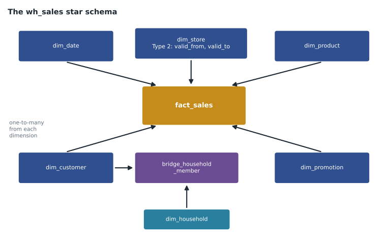
Data quality steps are frequent in items. Duplicates are found by grouping on the business key and counting, and resolved by keeping one row per key by a rule, such as the latest load. Missing keys in a fact table are mapped to an unknown member, such as product key −1, so that facts are not lost when a dimension row is missing. Nulls in measures are decided case by case: a null sale amount should be investigated or quarantined, not replaced with zero, while a null customer can mean a non-member sale. Type conversion is done with CAST or CONVERT in T-SQL, with cast() in PySpark, or with a change-type step in Power Query, and the item usually turns on doing it before a join so that keys match.
Query and analyze data
On the current outline, querying sits inside preparing data. Candidates should be able to query a lakehouse through its SQL analytics endpoint, query a warehouse with T-SQL or the visual query editor, and query an eventhouse with KQL. The SQL analytics endpoint is read-only for tables, but views, functions and stored procedures can be created in it, which lets a team expose a clean, documented layer without changing the tables. The visual query editor builds a query by dragging tables and steps, for analysts who do not write SQL. Cross-database queries can join a warehouse and a lakehouse endpoint in the same workspace by three-part names.
KQL was the biggest gap in Keiko's diagnostic. The essentials for this exam are short: a query starts with a table name and passes rows through operators joined by the pipe character; where filters, project chooses columns, extend adds calculated columns, summarize aggregates with by for grouping, and bin() groups timestamps into intervals. The query 'TillEvents | where Timestamp > ago(1h) | summarize Sales = sum(Amount) by bin(Timestamp, 5m), StoreId' reads as: from the till events of the last hour, total the sales in five-minute intervals by store. Lesson 7 practises reading KQL, SQL and DAX in more depth.
Optimize
The last group of skills is about finding and fixing slow loads and queries. In dataflows, the main tools are query folding, which pushes steps back to the source, and staging, which lands data before heavy transformations; a step that breaks folding early forces the dataflow to pull all the data first. In notebooks, the usual problems are too many small files, unnecessary shuffles and reading whole tables when a partition filter would do. In SQL, the usual problems are missing filters on large tables, functions on join columns and unnecessary SELECT * queries. The outline also names Delta table file sizes. Many small files slow every engine; OPTIMIZE compacts them, V-Order writes files in a layout that speeds reads, and partitioning helps only when queries filter on the partition column and each partition holds enough data, so partitioning a small table by day usually makes things worse.
Keiko's best example is the inventory adjustments table, which had 1,140 small files from frequent appends before an OPTIMIZE brought it down to a handful, and the 47-minute full sales load that became a 4-minute incremental load. Both are exactly the kind of before-and-after an exam item describes, asking which action caused the improvement or which to take first.
Views, functions and stored procedures
The outline asks candidates to create views, functions and stored procedures, and the item usually asks which one fits. A view is a saved SELECT statement that behaves like a table; it suits a clean, renamed layer over raw tables, such as vw_sales_current that hides closed Type 2 rows. An inline table-valued function is a view with parameters, such as fn_sales_for_region(@region), and it is also how a row-level security predicate is written in a warehouse. A stored procedure runs a series of statements, can change data and can take parameters; it suits a load step, such as usp_load_fact_sales, called from a pipeline. Views and functions can be created in both a warehouse and a lakehouse SQL analytics endpoint; stored procedures that change data need the warehouse, because the endpoint cannot write to tables.
Keiko had used views and stored procedures in wh_sales but had never created a view on a lakehouse endpoint, which is one of her seven skills not met. The difference matters on the exam: an item that says 'analysts must query cleaned lakehouse data with T-SQL, and the tables must not be changed' points to a view on the SQL analytics endpoint, not to a copy in a warehouse.
| Object | Takes parameters | Changes data | Lakehouse endpoint | Warehouse |
|---|---|---|---|---|
| View | No | No | Yes | Yes |
| Inline table-valued function | Yes | No | Yes | Yes |
| Stored procedure | Yes | Yes, in a warehouse | Yes, read-only work | Yes |
Loading patterns
Two loading patterns come up often. A full load replaces the whole table each run; it is simple and fits small dimensions. An incremental load brings only new or changed rows since the last run, using a watermark such as the highest modified date already loaded, and merges them into the target; it fits large fact tables. In a notebook, the merge is a Delta MERGE; in a warehouse, it is a MERGE statement or an UPDATE followed by an INSERT. Keiko's sales load moved from full to incremental in October, which is why it fell from 47 minutes to 4.
Worked problem
Choosing a partition column
A lakehouse table holds 96 million sales lines over seven years, about 6.4 GB. Most queries filter by sale year or by a date range within a year. Should the table be partitioned by day, by year, or not at all?
Show solution
- By day: about 7 × 365 = 2,555 partitions, an average of about 2.5 MB each. Far too small; it creates the small-file problem.
- By year: 7 partitions, about 0.9 GB each. Large enough, and most queries filter on year, so whole years can be skipped.
- Not at all: workable for 6.4 GB, but queries for one year must read file statistics for all of them.
- Year matches the common filter and gives large partitions, so it is the best of the three.
Answer: Partition by year; partitioning by day would create thousands of tiny partitions.
Common mistakes
MistakeUse a warehouse for every transformation because it has T-SQL.
InsteadChoose by skills and volume: dataflows for analysts, notebooks for large code-based work, T-SQL where the team and the target are in the warehouse.
MistakeWrite to a lakehouse table through its SQL analytics endpoint.
InsteadThe endpoint is read-only for tables; create views and functions there, or write with Spark, dataflows or pipelines.
MistakeDeleting a shortcut deletes the data it points to.
InsteadIt removes only the pointer.
MistakeReplace every null with zero.
InsteadDecide by meaning: a null sale amount needs investigation; a null customer may mean a non-member.
MistakePartition every table by date.
InsteadPartition only when queries filter on the column and partitions stay large.
MistakeChain a dataflow after a notebook by scheduling it later.
InsteadOrchestrate both from a pipeline so the second waits for the first.
Summary and key terms
- Lakehouses, warehouses and eventhouses all store data in OneLake; choose by engine, skills and latency.
- Shortcuts reference data without copying it; mirroring keeps a near-real-time copy of an operational database.
- Pipelines, dataflows and notebooks all ingest data; pipelines also orchestrate the others.
- Star schema skills include Type 1 and Type 2 dimensions, bridge tables, denormalizing, unknown members and handling duplicates and nulls.
- Query lakehouses through the read-only SQL analytics endpoint, warehouses with T-SQL or the visual query editor, and eventhouses with KQL.
- Optimize with query folding and staging in dataflows, fewer small files and partition filters in notebooks, and OPTIMIZE and V-Order on Delta tables.
- Lakehouse
- A Fabric item that stores files and Delta tables in OneLake, with a read-only SQL analytics endpoint.
- Warehouse
- A Fabric item with read-write T-SQL tables, views, functions and stored procedures.
- Eventhouse
- A Fabric item that holds KQL databases for streaming and time-series data.
- Shortcut
- A pointer from a lakehouse or KQL database to data stored elsewhere, read without copying.
- Slowly changing dimension
- A dimension that keeps history by overwriting (Type 1) or adding new rows (Type 2).
- Bridge table
- A table that links two tables in a many-to-many relationship.
- Query folding
- Power Query pushing transformation steps back to the source system.
Practice problems
Work each problem on paper first, then reveal the answer to check.
Which item suits a team that needs read-write tables through T-SQL?
Show answer
A warehouse.
What does a Type 2 change do to the old row?
Show answer
It closes it with an end date and marks it as no longer current.
Why map missing keys to an unknown member?
Show answer
So fact rows are not lost when a dimension row is missing.
What does bin(Timestamp, 5m) do in KQL?
Show answer
It groups timestamps into five-minute intervals.
Why is partitioning a small table by day usually harmful?
Show answer
It creates many tiny partitions and files.
Lesson quiz · 5 questions
Score 60% or more to complete this lesson.
Create a free account to save your progress, take quizzes and earn a certificate.