Gene flow, isolation by distance and admixture

Gene flow is the movement of alleles between populations through the dispersal of individuals or gametes. It opposes drift, which pushes populations apart, and it can either spread beneficial alleles or swamp local adaptation. Lesson 7 treated gene flow in the island model, where every population is equally connected to every other. Real organisms disperse over limited distances, so nearby populations exchange more migrants than distant ones. This lesson shows how gene flow is measured directly and indirectly, develops the theory of isolation by distance, introduces landscape genetics, and explains how genomic data reveal admixture between previously separated populations, including how admixture proportions and dates are estimated and how clustering methods should and should not be interpreted.

Measuring gene flow directly and indirectly

Direct methods track individuals or gametes. Mark–recapture and radio or satellite telemetry record where animals move; parentage analysis with genetic markers records where they actually breed, which is what matters genetically. Pollen and seed dispersal can be measured by assigning seedlings to their mother and father among genotyped adults. Direct methods give the dispersal kernel, the probability distribution of distances between birthplace and breeding site, but only over the few generations and the limited area that can be studied.

Indirect methods infer gene flow from the genetic structure it has produced. F_ST and the island model are one example. Indirect estimates integrate over many generations and capture rare long-distance events that direct studies miss, but they depend on model assumptions and confound current with historical gene flow. The two kinds of evidence often disagree, and the disagreements are informative: animals that move far but fail to breed contribute to direct estimates but not to gene flow, while a single successful long-distance migrant every few generations can be invisible to telemetry but decisive genetically.

Wright summarized the scale of local mating with the neighbourhood size. If σ² is the variance of the dispersal kernel along one axis and D is the density of breeding individuals, the effective number of individuals in a local mating neighbourhood in two dimensions is:

When N_b is small, below a few dozen, local drift is strong and populations become strongly structured over short distances even in continuous habitat. When it is in the thousands, a continuous population behaves almost as if it were panmictic over large areas.

Isolation by distance

If individuals disperse over short distances, genetic similarity should decline steadily with geographic distance, a pattern Wright called isolation by distance. François Rousset showed in 1997 that, in a two-dimensional continuous population at equilibrium, the quantity F_ST/(1 − F_ST) between pairs of local samples increases linearly with the logarithm of distance r, with a slope that depends only on the neighbourhood size:

In one dimension, as along a river or a coastline, the relationship is linear in distance itself. Rousset’s result is valuable because it allows Dσ², and hence the scale of dispersal, to be estimated from genetic data alone, and estimates obtained this way have matched direct estimates in several well-studied species. The pattern is tested by plotting genetic against geographic distance for all pairs of populations. Because the pairs are not independent (each population appears in many pairs), ordinary regression p-values are invalid. The Mantel test instead compares the observed correlation with correlations obtained after randomly permuting the population labels.

import numpy as np
rng = np.random.default_rng(322)

# a 1-D stepping-stone chain of 12 demes with migration to adjacent demes only
demes, N, m, loci, gens = 12, 60, 0.1, 400, 2500
p = np.full((demes, loci), 0.5)
for _ in range(gens):
    left = np.vstack([p[:1], p[:-1]]); right = np.vstack([p[1:], p[-1:]])
    p = (1 - m) * p + (m / 2) * (left + right)          # exchange with adjacent demes
    p = rng.binomial(2 * N, p) / (2 * N)                 # drift

def pair_fst(a, b):
    hw = a * (1 - a) + b * (1 - b)
    hb = a * (1 - b) + b * (1 - a)
    return 1 - hw.sum() / hb.sum()

i, j = np.triu_indices(demes, 1)
fst = np.array([pair_fst(p[a], p[b]) for a, b in zip(i, j)])
dist = (j - i).astype(float)
y = fst / (1 - fst)
slope, intercept = np.polyfit(dist, y, 1)
r_obs = np.corrcoef(dist, y)[0, 1]

# Mantel test: permute deme labels, recompute correlation
Y = np.zeros((demes, demes)); Y[i, j] = y; Y = Y + Y.T
count = 0
for _ in range(2000):
    perm = rng.permutation(demes)
    yp = Y[perm][:, perm][i, j]
    count += np.corrcoef(dist, yp)[0, 1] >= r_obs
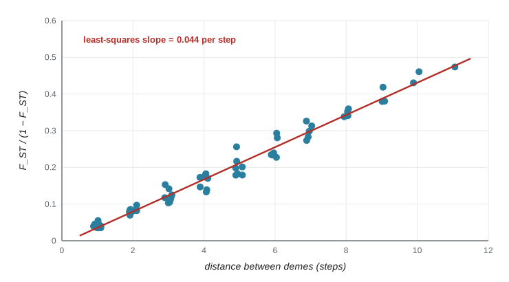
print(f"regression of FST/(1-FST) on distance: slope = {slope:.4f} per step")
print(f"Mantel r = {r_obs:.3f}, permutation p = {(count + 1) / 2001:.4f}")
print(f"one-dimensional theory: slope = 1/(4Nm) = {1 / (4 * N * m):.4f}")

regression of FST/(1-FST) on distance: slope = 0.0439 per step
Mantel r = 0.990, permutation p = 0.0005
one-dimensional theory: slope = 1/(4Nm) = 0.0417

The simulated chain shows a strong, significant increase of differentiation with distance. In one dimension, theory predicts a slope of 1/(4Dσ²), which for a stepping-stone chain with N individuals per deme and a fraction m dispersing to neighbours (so σ² = m steps²) is 1/(4Nm) per step. The simulated slope is close to this value, though the chain is short and has edges, so agreement is approximate.

Landscape genetics

Straight-line distance is often a poor measure of how hard it is for organisms to move. Landscape genetics replaces it with distances that account for habitat: least-cost paths through a map of resistance values, or resistance distances from circuit theory, which treat the landscape as an electrical circuit and account for multiple routes at once. Competing landscape models are compared by how well their distances predict genetic differentiation. Studies of this kind have shown, for example, that highways, reservoirs and urban areas act as barriers for many species, and have been used to locate wildlife crossings. Banff National Park’s overpasses and underpasses on the Trans-Canada Highway, among the most intensively studied in the world, were shown by genetic sampling of hair to allow grizzly and black bears from both sides of the highway to interbreed.

Clines, gradual changes in allele frequency across space, form where selection varies along an environmental gradient and dispersal mixes populations. BIOL-321 introduced the approximate width of a cline maintained by selection against migration, about σ/√s. Narrow clines can also form where two diverged populations meet and hybrids are less fit; such tension zones are held in place by a balance between dispersal and selection against hybrids and tend to settle in areas of low density. Comparing the widths and centres of clines at many loci across a hybrid zone is a powerful way to find genes involved in reproductive isolation, because loci under selection have narrower clines than neutral ones.

Admixture

Admixture is gene flow between populations that have been separated long enough to have diverged. If a population is formed by mixing two source populations in proportions α and 1 − α, the allele frequency at each locus in the first generation is simply p_h = αp_1 + (1 − α)p_2. With frequencies for both sources and the admixed population at many loci, α can be estimated by regression. In practice, ancestry proportions are estimated for each individual, because admixed individuals differ from one another.

Admixture also creates linkage disequilibrium. In the first generation, every individual carries whole chromosomes from one source or the other, so alleles that differ in frequency between the sources are associated along entire chromosomes. Each generation of recombination breaks the chromosomes into shorter ancestry tracts. After t generations, tracts from a source that contributed a proportion m of the ancestry have an average length of roughly 1/[(1 − m)t] Morgans, because a tract ends wherever a recombination event switches to the other ancestry, and the admixture LD between markers separated by d Morgans decays as e^(−dt). Fitting this decay to genome-wide data, as programs such as ALDER do, dates admixture events. These methods have dated, for example, admixture in many populations of the Americas to within the last 500 years, consistent with documented history, and Neanderthal admixture into the ancestors of non-Africans to roughly 50,000 years ago.

Patterson’s f-statistics provide formal tests. The f3 statistic f3(C; A, B) is the expected value of (p_C − p_A)(p_C − p_B) across loci. If population C is unadmixed, it tends to be positive; if C is a mixture of populations related to A and B, its allele frequencies are intermediate and f3 can be negative. A significantly negative f3 is therefore unambiguous evidence of admixture, though a positive value does not rule it out. Related four-population statistics, D and f4, test whether gene trees are shared asymmetrically and were used to detect Neanderthal and Denisovan ancestry in present-day humans, a story BIOL-321 told from the fossil side.

Clustering, PCA and their limits

Two exploratory methods dominate studies of population structure. Principal component analysis (PCA) of a genotype matrix finds the axes of greatest genetic variation. In 2008 John Novembre and colleagues showed that the first two principal components of genotypes from people across Europe reproduce a recognizable map of the continent, because isolation by distance makes genetic similarity track geography. Model-based clustering, as in the programs STRUCTURE (2000) and ADMIXTURE (2009), assumes the sample derives from K ancestral populations in Hardy–Weinberg equilibrium and estimates each individual’s ancestry proportions from each, using the same EM logic as the ABO estimation in lesson 2.

import numpy as np
rng = np.random.default_rng(3228)

# two invented source populations and a group with variable admixture proportions
L = 2000
anc = rng.uniform(0.05, 0.95, L)
F = 0.15
pA = rng.beta(anc * (1 - F) / F, (1 - anc) * (1 - F) / F)
pB = rng.beta(anc * (1 - F) / F, (1 - anc) * (1 - F) / F)
alpha = np.r_[np.ones(30), np.zeros(30), rng.uniform(0.2, 0.8, 40)]   # ancestry from A
P = alpha[:, None] * pA + (1 - alpha[:, None]) * pB
G = rng.binomial(2, P).astype(float)

# PCA on standardized genotypes
mu = G.mean(axis=0); sd = np.sqrt(mu / 2 * (1 - mu / 2)) + 1e-9
Z = (G - mu) / sd
U, S, Vt = np.linalg.svd(Z, full_matrices=False)
pc1 = U[:, 0] * S[0]
print(f"variance explained by PC1 = {S[0]**2 / np.sum(S**2):.3f}, PC2 = {S[1]**2 / np.sum(S**2):.3f}")

# estimate each admixed individual's ancestry by placing it on PC1 between the two source means
a_hat = (pc1 - pc1[30:60].mean()) / (pc1[:30].mean() - pc1[30:60].mean())
err = np.abs(a_hat[60:] - alpha[60:])
print(f"mean absolute error of PC1-based ancestry estimates: {err.mean():.3f}")

# k-means with K = 2 on PC1 and PC2 (illustrative only)
X = np.c_[pc1, U[:, 1] * S[1]]
cent = X[[0, 59]]
for _ in range(20):
    lab = np.argmin(((X[:, None, :] - cent[None]) ** 2).sum(axis=2), axis=1)
    cent = np.array([X[lab == k].mean(axis=0) for k in (0, 1)])
print("k-means splits the admixed individuals:", np.bincount(lab[60:], minlength=2))

variance explained by PC1 = 0.095, PC2 = 0.013
mean absolute error of PC1-based ancestry estimates: 0.025
k-means splits the admixed individuals: [21 19]

The simulation makes an important point. PCA places admixed individuals between the two sources in proportion to their ancestry, and PC1 alone recovers their admixture proportions well. A clustering method forced to choose K = 2 discrete groups, however, simply splits the admixed individuals between the two clusters according to which source they are closer to. Clusters are a property of the method and the chosen K, not proof that discrete populations exist. Clustering results are sensitive to sampling: if one region is sampled heavily and another lightly, the heavily sampled region tends to form its own cluster. And continuous variation produced by isolation by distance can be forced into apparently discrete clusters. Results from STRUCTURE-like programs should be reported for several values of K, interpreted alongside PCA and geography, and described as ancestry components, not as races or pure ancestral groups. In human genetics, the 2023 report of the US National Academies on population descriptors recommended against using race as a proxy for genetic ancestry for these reasons.