
BIOL-322 · Lesson 10 of 12 · 27 min
Detecting selection in molecular data
Natural selection leaves traces in DNA, and population genetics provides the null models needed to recognize them. BIOL-321 introduced the ratio of non-synonymous to synonymous substitution rates and the McDonald–Kreitman test as evidence that much protein evolution is adaptive. This lesson turns those ideas into working methods. We compute dN/dS from a pair of coding sequences, carry out the McDonald–Kreitman test with Fisher’s exact test and estimate the proportion of adaptive substitutions, discuss the biases that slightly deleterious mutations introduce, and then move from single genes to genome scans: F_ST outliers, the population branch statistic, haplotype-based statistics and time series from ancient DNA. Throughout, the central difficulty is the same: demography can mimic selection, so a signal is convincing only when it stands out against a genome-wide or simulated neutral background.
Synonymous and non-synonymous sites
In a protein-coding gene, some point mutations change the amino acid (non-synonymous) and some do not (synonymous), because of the redundancy of the genetic code. Synonymous changes are often close to neutral, so the synonymous substitution rate, dS, approximates the neutral mutation rate. The non-synonymous rate, dN, reflects both mutation and selection on the protein. Their ratio, ω = dN/dS, is the standard summary: ω well below 1 indicates purifying selection, ω near 1 is consistent with neutrality, and ω above 1 indicates that amino acid changes have been favoured repeatedly.
Computing ω requires counting sites as well as differences. A codon has three nucleotide positions, and each position is counted as partly synonymous and partly non-synonymous according to the fraction of possible changes at that position that leave the amino acid unchanged. The third position of a fourfold-degenerate codon, such as the last position of any glycine codon (GGN), is fully synonymous; the second position of almost every codon is fully non-synonymous. Summed over a typical gene, roughly a quarter of sites are synonymous and three quarters non-synonymous. Masatoshi Nei and Takashi Gojobori’s 1986 counting method divides the observed synonymous and non-synonymous differences by these site counts and then corrects for multiple hits with the Jukes–Cantor formula used in BIOL-321’s phylogenetics lesson.
import numpy as np

bases = "TCAG"
aas = "FFLLSSSSYY**CC*WLLLLPPPPHHQQRRRRIIIMTTTTNNKKSSRRVVVVAAAADDEEGGGG"
code = {a + b + c: aas[16*i + 4*j + k] for i, a in enumerate(bases)
        for j, b in enumerate(bases) for k, c in enumerate(bases)}

def syn_sites(codon):
    s = 0.0
    for pos in range(3):
        alts = [codon[:pos] + x + codon[pos+1:] for x in bases if x != codon[pos]]
        alts = [c for c in alts if code[c] != "*"]
        s += sum(code[c] == code[codon] for c in alts) / len(alts)
    return s

def nei_gojobori(seq1, seq2):
    # this simple version assumes codons differ at no more than one position
    S = N = Sd = Nd = 0.0
    for i in range(0, len(seq1), 3):
        c1, c2 = seq1[i:i+3], seq2[i:i+3]
        s = (syn_sites(c1) + syn_sites(c2)) / 2
        S += s; N += 3 - s
        if c1 != c2:
            if code[c1] == code[c2]: Sd += 1
            else: Nd += 1
    pS, pN = Sd / S, Nd / N
    jc = lambda p: -0.75 * np.log(1 - 4 * p / 3)
    return S, N, Sd, Nd, jc(pN) / jc(pS)

a = "ATGGCTCGTCTGAAAGGCTTCGATGAACTGAGCAAAGTTCGCCATTGGATCGGTCCAGAGCTTACCGGA"
b = "ATGGCCCGTCTGAAAGGTTTCGATGAGCTGAGCAGAGTCCGCCATTGGATCGGTCCAGAGCTTACCGGA"
S, N, Sd, Nd, omega = nei_gojobori(a, b)
print(f"synonymous sites = {S:.2f}, non-synonymous sites = {N:.2f}")
print(f"synonymous differences = {Sd:.0f}, non-synonymous differences = {Nd:.0f}")
print(f"dN/dS = {omega:.3f}")synonymous sites = 16.25, non-synonymous sites = 52.75 synonymous differences = 4, non-synonymous differences = 1 dN/dS = 0.064
The invented pair differs at five positions, four of them synonymous third-position changes and one an amino acid change, so ω is far below 1, the typical signature of purifying selection. Real analyses average ω over many genes or estimate it with likelihood models of codon evolution, such as those in the PAML and HyPhy packages. These allow ω to vary among sites, among branches of a phylogeny, or both. Because adaptive change usually affects only a few sites in a protein over a short period, a gene-wide average ω rarely exceeds 1 even when adaptation has occurred; site and branch-site models are designed to find the few codons or lineages with ω above 1, as in the antigen-binding sites of major histocompatibility complex genes or the surface proteins of influenza viruses.
The McDonald–Kreitman test in practice
John McDonald and Martin Kreitman’s 1991 test compares two ratios within one gene. Polymorphisms within a species, P_N and P_S, and fixed differences between species, D_N and D_S, are counted separately for non-synonymous and synonymous sites. Under neutrality, both kinds of site should contribute to polymorphism and divergence in the same proportion, so P_N/P_S should equal D_N/D_S. An excess of non-synonymous fixed differences indicates that positive selection has fixed amino acid changes. Because the test compares the two classes of site within the same gene and the same genealogy, it is robust to most demographic history, its main advantage over Tajima’s D.
The 2 × 2 table is analysed with Fisher’s exact test, which computes the probability of the observed table, and all more extreme tables, given the row and column totals. The proportion of non-synonymous substitutions driven by positive selection, α, was defined by Nicolas Smith and Adam Eyre-Walker in 2002, and the neutrality index, NI, summarizes the direction of departure:
Worked problem
The alcohol dehydrogenase data
McDonald and Kreitman’s original Adh data from Drosophila melanogaster and its relatives had D_N = 7, D_S = 17, P_N = 2 and P_S = 42. Calculate α and NI.
Show solution
- D_N/D_S = 7/17 ≈ 0.41; P_N/P_S = 2/42 ≈ 0.048.
- NI = 0.048/0.41 ≈ 0.12, far below 1, meaning an excess of non-synonymous divergence.
- α = 1 − (17 × 2)/(7 × 42) = 1 − 34/294 ≈ 0.88.
- Fisher’s exact test on the table gives p ≈ 0.007 (see the code below).
Answer: α ≈ 0.88: on this estimate, most amino acid substitutions in Adh between these species were driven by positive selection.
import numpy as np
from scipy.stats import fisher_exact
from scipy.optimize import curve_fit

def mk(Dn, Ds, Pn, Ps):
    odds, p = fisher_exact([[Dn, Ds], [Pn, Ps]])
    alpha = 1 - (Ds * Pn) / (Dn * Ps)
    NI = (Pn / Ps) / (Dn / Ds)
    return alpha, NI, p

print("Adh (McDonald and Kreitman 1991): alpha = %.2f, NI = %.2f, Fisher p = %.4f" % mk(7, 17, 2, 42))

# effect of slightly deleterious polymorphisms: invented counts by derived allele frequency class
freq = np.array([0.05, 0.15, 0.25, 0.35, 0.45, 0.55, 0.65, 0.75, 0.85])
Pn = np.array([130, 50, 28, 18, 14, 11, 9, 8, 7])
Ps = np.array([200, 100, 66, 50, 40, 33, 28, 25, 22])
Dn, Ds = 50, 100
alpha_x = 1 - (Ds / Dn) * (Pn / Ps)
for f, a in zip(freq[[0, 2, 4, 8]], alpha_x[[0, 2, 4, 8]]):
    print(f"alpha using polymorphisms near frequency {f:.2f}: {a:+.2f}")
print(f"alpha with all polymorphisms pooled: {1 - (Ds / Dn) * Pn.sum() / Ps.sum():+.2f}")
curve = lambda x, a, b, c: a + b * np.exp(-c * x)
(a, b, c), _ = curve_fit(curve, freq, alpha_x, p0=(0.4, -1, 5), maxfev=10000)
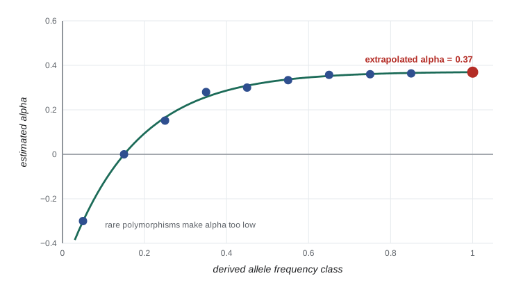
print(f"asymptotic alpha (exponential fit extrapolated to frequency 1): {curve(1, a, b, c):+.2f}")Adh (McDonald and Kreitman 1991): alpha = 0.88, NI = 0.12, Fisher p = 0.0073 alpha using polymorphisms near frequency 0.05: -0.30 alpha using polymorphisms near frequency 0.25: +0.15 alpha using polymorphisms near frequency 0.45: +0.30 alpha using polymorphisms near frequency 0.85: +0.36 alpha with all polymorphisms pooled: +0.02 asymptotic alpha (exponential fit extrapolated to frequency 1): +0.37
The second part of the code addresses an important bias. Slightly deleterious non-synonymous mutations can drift to low frequency and contribute to polymorphism, but they rarely become fixed. They inflate P_N and so make α too low, sometimes even negative. Rare polymorphisms are the most affected. One remedy is to exclude polymorphisms below a frequency threshold; a better one, the asymptotic McDonald–Kreitman method proposed by Philipp Messer and Dmitri Petrov in 2013, calculates α separately for each frequency class, fits a curve of the form a + b e^(−cx) and extrapolates it to x = 1, the frequency of fixation. In the invented data, α estimated from rare polymorphisms is negative, α from all polymorphisms pooled is close to zero, and α from common polymorphisms is much higher; the extrapolated value is the best estimate of the true proportion of adaptive substitutions. Applied across genomes, such methods suggest that around half of amino acid substitutions in Drosophila were adaptive, while estimates for humans are much lower, consistent with the nearly neutral theory’s prediction that selection is less efficient in species with smaller N_e.
Scanning genomes for local adaptation
Selection that differs among populations increases differentiation at the loci involved. Richard Lewontin and Jesse Krakauer proposed in 1973 that loci with unusually high F_ST compared with the rest of the genome could be candidates for local adaptation. The idea is sound, but the null distribution of F_ST depends strongly on demography: bottlenecks, hierarchical structure and range expansions all produce long tails of high F_ST at neutral loci. Modern outlier methods, such as those implemented in BayeScan, OutFLANK and pcadapt, model the neutral distribution more carefully, and genotype–environment association methods test whether allele frequencies correlate with environmental variables more than expected given population structure.
The population branch statistic (PBS) uses three populations to locate where along a tree a frequency change happened. Pairwise F_ST values are converted into branch lengths, T = −ln(1 − F_ST), and the length of the branch leading to the focal population is:
A large PBS means that the focal population has diverged unusually far from both comparison populations at that locus. Xin Yi and colleagues used it in 2010 to compare Tibetans with Han Chinese and Danes, and the strongest signal in the genome was at EPAS1, a gene in the hypoxia-response pathway. Later work found that the Tibetan EPAS1 haplotype was introgressed from Denisovans, an example of adaptive introgression. Comparable studies have found signals of high-altitude adaptation in Andean populations at different genes, a reminder that the same environmental challenge can be met by different genetic routes.
import numpy as np
rng = np.random.default_rng(322)

L = 5000
anc = rng.uniform(0.1, 0.9, L)
def drift(p, F):
    a = p * (1 - F) / F; b = (1 - p) * (1 - F) / F
    return rng.beta(a, b)
pAB = drift(anc, 0.02)                      # ancestor of A and B
pA = drift(pAB, 0.03); pB = drift(pAB, 0.03); pC = drift(anc, 0.08)
pA[:10] = np.clip(pA[:10] + 0.5, 0, 0.99)   # ten invented loci under selection in population A

def fst(p, q):
    hw = p * (1 - p) + q * (1 - q); hb = p * (1 - q) + q * (1 - p)
    return 1 - hw / hb
T = lambda p, q: -np.log(1 - np.clip(fst(p, q), 0, 0.999))
pbs = (T(pA, pB) + T(pA, pC) - T(pB, pC)) / 2
cut = np.quantile(pbs, 0.999)
top = np.argsort(pbs)[::-1][:10]
print(f"99.9th percentile of PBS = {cut:.3f}")
print(f"selected loci among the top 10 PBS values: {np.sum(top < 10)} of 10")
print(f"median PBS at selected loci = {np.median(pbs[:10]):.3f}; genome-wide median = {np.median(pbs):.3f}")99.9th percentile of PBS = 0.388 selected loci among the top 10 PBS values: 8 of 10 median PBS at selected loci = 0.398; genome-wide median = 0.004
Time series from ancient DNA
Most tests infer selection indirectly from present-day patterns. Ancient DNA allows allele frequency trajectories to be observed directly. Since Iain Mathieson and colleagues’ 2015 study of 230 ancient Europeans, samples of thousands of ancient genomes have tracked changes at loci for pigmentation, diet, immunity and height across the last 10,000 years. An allele whose frequency changes faster than drift could plausibly explain, given the effective size, is a candidate for selection. The lactase persistence allele, rising from near zero to high frequency in northern Europe within a few thousand years, is again the clearest example. Time-series analyses must account for population replacement and admixture, which also change allele frequencies quickly, so they compare each locus with the genome-wide pattern of ancestry change.
Validating candidates
A statistical signal is only the beginning. A convincing case for adaptation combines several kinds of evidence: a population-genetic signal that is robust to plausible demographic models; a functional variant with a demonstrated effect on a molecular or organismal phenotype; and an ecological reason why that phenotype would affect fitness in the relevant environment. Examples meeting all three criteria include lactase persistence, the Duffy-null allele that protects against Plasmodium vivax malaria, the threespine stickleback Eda allele that reduces armour plating in freshwater, and the melanocortin-1 receptor variants that give light coats to beach mice on pale sand. For many genome-scan candidates, the functional and ecological steps are still missing.
| Approach | Timescale | Signal | Main confounder |
|---|---|---|---|
| dN/dS (site and branch models) | Millions of years | Excess amino acid substitution | Saturation of synonymous sites; selection on codon usage |
| McDonald–Kreitman test | Since species divergence | Excess non-synonymous divergence relative to polymorphism | Slightly deleterious polymorphisms; changes in N_e |
| Tajima’s D and SFS tests | Up to about 4N_e generations | Excess rare or intermediate variants | Demographic history |
| F_ST outliers, PBS | Since population split | Unusual differentiation | Hierarchical structure; bottlenecks |
| EHH and iHS | Recent, ongoing | Long haplotypes for allele frequency | Variation in recombination rate |
| Ancient DNA time series | Last 10,000 years or so | Frequency change faster than drift | Population replacement and admixture |
Common mistakes
MistakeExpecting a gene-wide dN/dS above 1 whenever a protein has adapted.
InsteadAdaptation usually affects a few sites briefly; use site or branch-site models.
MistakeIgnoring slightly deleterious polymorphisms in the McDonald–Kreitman test.
InsteadThey inflate P_N and bias α downward; exclude rare variants or use the asymptotic method.
MistakeCalling the top 1 per cent of F_ST values ‘selected genes’.
InsteadEvery genome has a top 1 per cent; compare against a demographic null model and seek functional evidence.
MistakeTreating Tajima’s D and the McDonald–Kreitman test as equally sensitive to demography.
InsteadMK compares site classes within one gene and is far more robust to demography than D.
MistakeConsidering a statistical outlier proof of adaptation.
InsteadCombine population-genetic, functional and ecological evidence.
Summary and key terms
- ω = dN/dS compares non-synonymous and synonymous substitution rates; site and branch-site models find episodes of positive selection.
- The McDonald–Kreitman test compares P_N/P_S with D_N/D_S using Fisher’s exact test; α = 1 − D_S P_N/(D_N P_S).
- Slightly deleterious polymorphisms bias α downward; the asymptotic MK method extrapolates across frequency classes.
- F_ST outliers and the population branch statistic locate local adaptation, as at EPAS1 in Tibetans.
- Ancient DNA time series observe allele frequency change directly but must account for population turnover.
- Convincing evidence of adaptation combines population-genetic, functional and ecological lines.
- synonymous substitution
- A nucleotide change that does not alter the encoded amino acid.
- non-synonymous substitution
- A nucleotide change that alters the encoded amino acid.
- dN/dS
- The ratio of non-synonymous to synonymous substitution rates per site, ω.
- McDonald–Kreitman test
- A test comparing polymorphism and divergence at synonymous and non-synonymous sites.
- Fisher’s exact test
- A test of association in a 2 × 2 table using the exact hypergeometric distribution.
- neutrality index
- NI = (P_N/P_S)/(D_N/D_S); values below 1 suggest positive selection.
- α (alpha)
- The estimated proportion of non-synonymous substitutions fixed by positive selection.
- population branch statistic
- A three-population measure of allele frequency change on the branch to a focal population.
- adaptive introgression
- Acquisition of a beneficial allele through hybridization with another population or species.
- genotype–environment association
- Testing whether allele frequencies correlate with environmental variables beyond the effect of structure.
Practice problems
Work each problem on paper first, then reveal the answer to check.
What does ω = 0.05 indicate?
Show answer
Strong purifying selection: most amino acid changes are removed.
What fraction of the third position of a fourfold-degenerate codon is synonymous?
Show answer
All of it (1 full site).
A gene has D_N = 20, D_S = 30, P_N = 10 and P_S = 60. Calculate α.
Show answer
1 − (30 × 10)/(20 × 60) = 1 − 0.25 = 0.75.
Calculate NI for the same gene.
Show answer
(10/60)/(20/30) = 0.167/0.667 = 0.25.
What statistical test is used on the MK 2 × 2 table?
Show answer
Fisher’s exact test, or a G-test with large counts.
Why can α be negative?
Show answer
Slightly deleterious non-synonymous polymorphisms inflate P_N relative to D_N.
F_ST values are 0.10 (A–B), 0.30 (A–C) and 0.20 (B–C). Calculate PBS for A.
Show answer
T = 0.105, 0.357, 0.223; PBS = (0.105 + 0.357 − 0.223)/2 ≈ 0.12.
Why are F_ST outliers not automatically selected loci?
Show answer
Demography produces long tails of F_ST at neutral loci.
What made EPAS1 in Tibetans an example of adaptive introgression?
Show answer
The adaptive haplotype was inherited from Denisovans.
Name three lines of evidence needed for a convincing case of adaptation.
Show answer
A robust population-genetic signal, a functional effect of the variant and an ecological reason for its fitness effect.
Lesson quiz · 5 questions
Score 60% or more to complete this lesson.
Create a free account to save your progress, take quizzes and earn a certificate.