
BIOL-322 · Lesson 2 of 12 · 32 min
Hardy–Weinberg, multiple alleles and estimating allele frequencies
The Hardy–Weinberg principle is the null model of population genetics. It states that, in a large population with random mating and no selection, mutation or migration, allele frequencies do not change from one generation to the next and genotype frequencies settle into the proportions p², 2pq and q² after a single generation of random mating. BIOL-201 used these proportions with a chi-square test as a quality check on genotype data. This lesson goes further in three directions: it extends the principle to loci with many alleles and to sex-linked loci; it shows how to estimate allele frequencies when some genotypes cannot be distinguished, using the expectation–maximization (EM) algorithm on the ABO blood groups; and it replaces the chi-square approximation with an exact test that remains valid for rare alleles and small samples.
Why the proportions arise
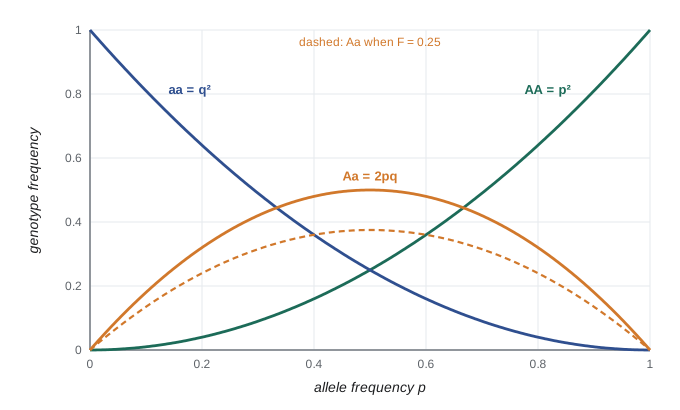
The principle follows from a simple observation. Under random mating, the two gene copies that unite to form a zygote are drawn independently from the population’s pool of gametes. If allele A makes up a fraction p of that pool, the chance that both copies are A is p × p, the chance that both are a is q × q, and the chance of one of each is 2pq, the factor of 2 counting the two ways the heterozygote can form. Because each genotype passes on its alleles in proportion to its genotype, the allele frequency in the next gamete pool is p² + pq = p(p + q) = p. Nothing changes.
The assumptions are worth listing because each is the subject of a later lesson. Selection (lesson 3) changes allele frequencies by differential survival and reproduction. Finite population size (lesson 4) causes drift. Mutation (lesson 5) introduces new alleles. Non-random mating and population structure (lesson 7) change genotype frequencies even when allele frequencies stay fixed. Migration (lesson 8) mixes populations with different frequencies. The power of the Hardy–Weinberg principle is that it isolates these forces: any departure from the expected proportions is a clue that one of them is at work, or that the data contain errors.
Multiple alleles
With k alleles at frequencies p_1, p_2, … , p_k, random union of gametes gives homozygotes A_iA_i at frequency p_i² and heterozygotes A_iA_j at frequency 2p_ip_j. There are k homozygote classes and k(k − 1)/2 heterozygote classes. For a microsatellite with 15 alleles, that is 15 homozygotes and 105 heterozygotes, so many genotype classes have expected counts far below one even in a sample of several hundred individuals. This is the main reason the chi-square approximation fails for highly polymorphic loci.
The total expected heterozygosity is 1 − Σp_i², the H_e of lesson 1. With many alleles at similar frequencies, H_e approaches 1, and nearly every individual is heterozygous. This is exactly why forensic laboratories use highly polymorphic STR loci: two unrelated people are very unlikely to share a genotype at any one locus, and the probabilities multiply across loci, as lesson 12 shows.
Worked problem
Expected genotypes at a three-allele locus
A locus has alleles A1, A2 and A3 at frequencies 0.5, 0.3 and 0.2. In a random-mating population of 1,000, how many individuals of each genotype are expected?
Show solution
- Homozygotes: A1A1 = 0.25 × 1,000 = 250; A2A2 = 0.09 × 1,000 = 90; A3A3 = 0.04 × 1,000 = 40.
- Heterozygotes: A1A2 = 2 × 0.5 × 0.3 × 1,000 = 300; A1A3 = 2 × 0.5 × 0.2 × 1,000 = 200; A2A3 = 2 × 0.3 × 0.2 × 1,000 = 120.
- Check: 250 + 90 + 40 + 300 + 200 + 120 = 1,000.
- Expected heterozygosity: (300 + 200 + 120)/1,000 = 0.62 = 1 − (0.25 + 0.09 + 0.04).
Answer: 250, 90 and 40 homozygotes and 300, 200 and 120 heterozygotes; 62 per cent of the population is expected to be heterozygous.
Sex-linked loci and the approach to equilibrium
For an X-linked locus in a species where females are XX and males XY, females carry two copies and males one. Males inherit their single X from their mothers, while females inherit one X from each parent. If allele frequencies differ between the sexes, say p_f in females and p_m in males, then in the next generation the male frequency equals the previous female frequency, and the female frequency is the average of the previous male and female frequencies:
The difference between the sexes halves and changes sign every generation, so the two frequencies oscillate as they converge on the overall frequency (2p_f + p_m)/3. Unlike an autosomal locus, an X-linked locus therefore needs several generations to reach equilibrium after a disturbance such as the mixing of two populations. At equilibrium, the frequency of a recessive X-linked trait in males equals q, while in females it is q². This is why red–green colour vision deficiency, with q of about 0.08 in many populations of European ancestry, affects about 8 per cent of men but well under 1 per cent of women.
Estimating allele frequencies when genotypes are hidden: the ABO system
Counting alleles is simple when every genotype can be identified. The ABO blood group is the classic case where it cannot. Alleles A and B are codominant to each other and both are dominant to O, so the six genotypes produce only four phenotypes: type A (AA or AO), type B (BB or BO), type AB and type O (OO). Given counts of the four phenotypes, how should the three allele frequencies be estimated?
The answer is maximum likelihood, and the most convenient way to find the maximum is the EM algorithm. The idea is to alternate two steps. In the expectation step, we use the current guess of allele frequencies to split each ambiguous phenotype into its expected genotype counts: of the type A people, a fraction p_A²/(p_A² + 2p_Ap_O) are expected to be AA and the rest AO. In the maximization step, we count alleles in the reconstructed genotypes, exactly as if they had been observed, to get new frequency estimates. Repeating the two steps increases the likelihood at every iteration and converges to the maximum likelihood estimates.
import numpy as np

# invented phenotype counts for a sample of 1,000 blood donors
nA, nB, nAB, nO = 421, 106, 37, 436
n = nA + nB + nAB + nO

pA, pB, pO = 1/3, 1/3, 1/3                     # starting guess
for it in range(1, 101):
    # E step: split ambiguous phenotypes into expected genotype counts
    nAA = nA * pA**2 / (pA**2 + 2*pA*pO); nAO = nA - nAA
    nBB = nB * pB**2 / (pB**2 + 2*pB*pO); nBO = nB - nBB
    # M step: count alleles
    new = np.array([2*nAA + nAO + nAB, 2*nBB + nBO + nAB, 2*nO + nAO + nBO]) / (2*n)
    if np.max(np.abs(new - [pA, pB, pO])) < 1e-10:
        break
    pA, pB, pO = new
print(f"converged after {it} iterations")
print(f"pA = {pA:.4f}, pB = {pB:.4f}, pO = {pO:.4f}")

# expected phenotype counts under these estimates, and a goodness-of-fit check
exp = n * np.array([pA**2 + 2*pA*pO, pB**2 + 2*pB*pO, 2*pA*pB, pO**2])
obs = np.array([nA, nB, nAB, nO])
chi2 = np.sum((obs - exp)**2 / exp)
print("expected A, B, AB, O:", np.round(exp, 1))
print(f"chi-square = {chi2:.2f} on 1 degree of freedom")converged after 13 iterations pA = 0.2640, pB = 0.0743, pO = 0.6617 expected A, B, AB, O: [419.1 103.9 39.2 437.8] chi-square = 0.19 on 1 degree of freedom
The algorithm converges in a handful of iterations. The goodness-of-fit test has only one degree of freedom: four phenotype classes, minus one because the counts sum to n, minus two for the two independent allele frequencies estimated. A quick alternative estimator, Bernstein’s method, uses the square root of the O frequency as p_O, but it does not force the three estimates to sum to 1 and is less efficient. The EM approach generalizes far beyond blood groups: the same logic is used to infer haplotype frequencies from unphased genotypes (lesson 9), to estimate admixture proportions (lesson 8) and to call genotypes from low-coverage sequencing data.
Worked problem
One EM iteration by hand
With current estimates p_A = 0.3, p_B = 0.1 and p_O = 0.6, how are 300 type A people split into AA and AO genotypes in the E step?
Show solution
- p_A² = 0.09; 2p_Ap_O = 2 × 0.3 × 0.6 = 0.36. Total = 0.45.
- Expected AA = 300 × 0.09/0.45 = 60.
- Expected AO = 300 × 0.36/0.45 = 240.
- These 60 AA and 240 AO individuals contribute 2 × 60 + 240 = 360 A alleles and 240 O alleles in the M step.
Answer: 60 AA and 240 AO; most type A people are heterozygous because O is common.
Testing Hardy–Weinberg proportions exactly
The familiar chi-square test compares observed and expected genotype counts. It relies on a large-sample approximation that breaks down when any expected count is small, which is common for rare alleles or highly polymorphic loci. For a biallelic locus there is a better option: the exact test. Conditional on the observed number of each allele, the number of heterozygotes in a sample of n individuals has a known probability distribution under Hardy–Weinberg proportions, first written down by Howard Levene in 1949:
Here n_A and n_B are the allele counts. The p-value is the sum of the probabilities of all heterozygote counts that are as likely as, or less likely than, the observed count. Janis Wigginton and colleagues published a fast algorithm in 2005 that made this test standard for genome-wide SNP data. The code below implements it by enumerating every possible heterozygote count, which is fast enough for any realistic sample.
import numpy as np
from scipy.special import gammaln
from scipy.stats import chi2

def hwe_exact(n_AA, n_AB, n_BB):
    n = n_AA + n_AB + n_BB
    nA = 2*n_AA + n_AB; nB = 2*n - nA
    rare = min(nA, nB)
    het = np.arange(rare % 2, rare + 1, 2)      # heterozygote counts with the right parity
    hom_r = (rare - het) // 2; hom_c = n - het - hom_r
    logp = (gammaln(n+1) - gammaln(hom_r+1) - gammaln(het+1) - gammaln(hom_c+1)
            + het*np.log(2) + gammaln(nA+1) + gammaln(nB+1) - gammaln(2*n+1))
    probs = np.exp(logp)
    p_obs = probs[het == n_AB][0]
    return probs[probs <= p_obs * (1 + 1e-7)].sum()

def hwe_chi2(n_AA, n_AB, n_BB):
    n = n_AA + n_AB + n_BB; p = (2*n_AA + n_AB) / (2*n)
    exp = n * np.array([p**2, 2*p*(1 - p), (1 - p)**2])
    x = np.sum((np.array([n_AA, n_AB, n_BB]) - exp)**2 / exp)
    return chi2.sf(x, 1)

for g in [(57, 36, 7), (88, 10, 2), (95, 3, 2), (40, 20, 40)]:
print(f"AA, AB, BB = {g}: exact p = {hwe_exact(*g):.3g}, chi-square p = {hwe_chi2(*g):.3g}")AA, AB, BB = (57, 36, 7): exact p = 0.789, chi-square p = 0.689 AA, AB, BB = (88, 10, 2): exact p = 0.0654, chi-square p = 0.0204 AA, AB, BB = (95, 3, 2): exact p = 0.00265, chi-square p = 2.72e-08 AA, AB, BB = (40, 20, 40): exact p = 7.9e-10, chi-square p = 1.97e-09
For the first genotype set, a common allele in good agreement with expectation, the two tests broadly agree. In the second and third sets, the rare allele appears in only 14 and 7 gene copies. In the second set the chi-square test would declare a significant departure at the 5 per cent level when the exact test does not, and in the third it exaggerates the evidence against Hardy–Weinberg proportions by a large factor because the expected number of BB homozygotes is tiny. The exact test gives a reliable answer. The last set shows a strong heterozygote deficit, which both tests detect easily.
Interpreting departures
A significant departure from Hardy–Weinberg proportions is a symptom, not a diagnosis. A deficit of heterozygotes can result from inbreeding, from population structure (the Wahlund effect of lesson 7), from assortative mating, from selection against heterozygotes or, very often, from technical problems such as null alleles that fail to amplify or from low-coverage sequencing that misses one allele. An excess of heterozygotes can result from selection favouring heterozygotes, from sampling a recent mixture of two populations, from very small numbers of breeders (when allele frequencies happen to differ between the sexes), or from paralogous sequences that are mistakenly merged so that two loci look like one heterozygous locus.
A useful summary of the direction and size of a departure is the fixation index F = 1 − H_o/H_e. Positive F means fewer heterozygotes than expected; negative F means more. Under inbreeding, genotype frequencies become p² + Fpq, 2pq(1 − F) and q² + Fpq. Because inbreeding affects every locus in the genome while technical artefacts and selection affect particular loci, a consistent positive F across many loci points to the mating system or population structure, whereas an extreme F at a handful of loci points to the loci themselves.
| Pattern across loci | Most likely explanations | Next step |
|---|---|---|
| Heterozygote deficit at most loci | Inbreeding, selfing, or a sample that combines several populations | Estimate F; look for structure with F-statistics or clustering |
| Heterozygote deficit at a few loci only | Null alleles, allele dropout, poor genotype calls | Check call quality; redesign primers or drop loci |
| Heterozygote excess at a few loci | Merged paralogues, copy-number variants, rarely balancing selection | Check read depth and allele balance |
| Heterozygote excess at most loci | Very few breeders, recent admixture of two diverged groups | Check sample origin and pedigree |
In genome-wide studies, each of hundreds of thousands of SNPs is tested, so a p-value threshold of 0.05 would flag thousands of loci by chance alone. Quality-control pipelines therefore use very stringent thresholds, such as p below 10⁻⁶ in controls, and test only in a group that should be in equilibrium. In case–control studies, a departure confined to cases can itself be a sign of association with disease, so filtering on cases would remove real signals.
Worked problem
Estimating F from heterozygosity
In a self-compatible plant, a sample of 200 individuals at a SNP with p = 0.4 contains 60 heterozygotes. Estimate F and the expected genotype counts under that F.
Show solution
- Expected heterozygosity 2pq = 2 × 0.4 × 0.6 = 0.48; expected count 96.
- F = 1 − H_o/H_e = 1 − (60/200)/0.48 = 1 − 0.30/0.48 = 0.375.
- Homozygote AA expected frequency = p² + Fpq = 0.16 + 0.375 × 0.24 = 0.25, so 50 plants.
- Homozygote aa = q² + Fpq = 0.36 + 0.09 = 0.45, so 90 plants. Heterozygotes = 0.48 × 0.625 × 200 = 60.
Answer: F ≈ 0.375, consistent with substantial self-fertilization if the pattern holds across loci; expected counts 50 AA, 60 Aa and 90 aa.
For a plant population that reproduces partly by selfing at rate S, the equilibrium inbreeding coefficient is F = S/(2 − S). An F of 0.375 implies S of about 0.55, so roughly half of seeds would come from self-fertilization. Estimates of this kind are routine in plant breeding and in conservation genetics of rare plants.
Common mistakes
MistakeUsing the chi-square test when some expected genotype counts are below about 5.
InsteadUse the exact test, which is valid for any sample size and allele frequency.
MistakeConcluding that a population is inbred because one locus deviates from Hardy–Weinberg proportions.
InsteadLook across many loci. Inbreeding affects the whole genome; single-locus departures more often reflect technical problems or selection.
MistakeEstimating ABO allele frequencies by counting type A people as AA.
InsteadType A includes AO heterozygotes; use the EM algorithm or another maximum likelihood method.
MistakeExpecting an X-linked locus to reach equilibrium after one generation of random mating.
InsteadSex differences in frequency oscillate and halve each generation, so equilibrium takes several generations.
MistakeFiltering SNPs for Hardy–Weinberg departures in disease cases.
InsteadFilter in controls; departures in cases can reflect true association.
Summary and key terms
- Random union of gametes gives Hardy–Weinberg proportions after one generation; each assumption broken points to a different evolutionary force.
- With k alleles, homozygotes occur at p_i² and heterozygotes at 2p_ip_j; many classes have tiny expected counts.
- At X-linked loci, sex differences in allele frequency halve and alternate in sign each generation.
- The EM algorithm finds maximum likelihood allele frequencies when genotypes are hidden, as in the ABO system.
- The exact test of Hardy–Weinberg proportions conditions on allele counts and remains valid for rare alleles.
- The fixation index F = 1 − H_o/H_e measures the size and direction of a departure; its pattern across loci helps diagnose its cause.
- Hardy–Weinberg proportions
- The genotype frequencies p², 2pq and q² expected under random mating with no other forces.
- codominance
- Both alleles are expressed in the heterozygote, as for A and B in the ABO system.
- maximum likelihood
- Choosing parameter values that make the observed data most probable.
- EM algorithm
- An iterative method that alternates estimating hidden data and re-estimating parameters to find maximum likelihood estimates.
- exact test
- A test that computes p-values from the exact sampling distribution instead of a large-sample approximation.
- fixation index
- F = 1 − H_o/H_e, the proportional deficit of heterozygotes relative to expectation.
- null allele
- An allele that fails to amplify or be detected, making heterozygotes appear homozygous.
- selfing
- Self-fertilization, the most extreme form of inbreeding.
- X-linked locus
- A gene on the X chromosome, present in two copies in females and one in males in XY species.
- paralogue
- A gene copy produced by duplication within a genome, which can be mistaken for an allele.
Practice problems
Work each problem on paper first, then reveal the answer to check.
How many genotypes are possible at a locus with 6 alleles?
Show answer
6 homozygotes + 15 heterozygotes = 21.
Alleles have frequencies 0.7, 0.2 and 0.1. What is the expected frequency of A1A3 heterozygotes?
Show answer
2 × 0.7 × 0.1 = 0.14.
At an X-linked locus, p_f = 0.6 and p_m = 0.2. What are the frequencies in the next generation?
Show answer
p_m = 0.6; p_f = (0.2 + 0.6)/2 = 0.4.
If 9 per cent of men have an X-linked recessive trait, what fraction of women are expected to have it?
Show answer
q = 0.09, so q² ≈ 0.0081, or about 0.8 per cent.
In an E step with p_B = 0.1 and p_O = 0.6, what fraction of type B people are expected to be BB?
Show answer
0.01/(0.01 + 0.12) ≈ 0.077.
How many degrees of freedom does a goodness-of-fit test for ABO phenotypes have?
Show answer
One: four classes minus one minus two estimated frequencies.
Why can the chi-square HWE test mislead for rare alleles?
Show answer
Expected counts of rare homozygotes are tiny, so the approximation is poor and p-values can be far too small.
A population has H_o = 0.30 and H_e = 0.40. What is F?
Show answer
1 − 0.30/0.40 = 0.25.
What selfing rate gives an equilibrium F of 0.5?
Show answer
F = S/(2 − S) = 0.5 gives S = 2/3.
Name two technical causes of an apparent heterozygote excess.
Show answer
Merged paralogous loci and copy-number variants that make one locus look like two alleles.
Lesson quiz · 5 questions
Score 60% or more to complete this lesson.
Create a free account to save your progress, take quizzes and earn a certificate.