
BIOL-322 · Lesson 11 of 12 · 26 min
Quantitative genetics, QTL and GWAS
Most traits that matter in agriculture, medicine and ecology, such as height, yield, blood pressure, flowering time and disease risk, vary continuously and are influenced by many genes and by the environment. BIOL-321 estimated heritability from relatives and used the breeder’s equation to predict responses to selection, treating genes as a black box. This lesson opens the box. It connects the variance components of quantitative genetics to allele frequencies and effects at individual loci, explains how quantitative trait loci are mapped in experimental crosses, and describes how genome-wide association studies (GWAS) test millions of variants in natural populations. It ends with polygenic scores: what they can and cannot predict, why their accuracy depends on how closely a person’s genetic ancestry matches the people in the original study, and why none of this supports essentialist ideas about human groups.
From one locus to variance components
Consider a locus with alleles A1 and A2 at frequencies p and q that affects a trait. Assign genotypic values +a to A1A1, d to A1A2 and −a to A2A2, so that a measures the additive effect and d the dominance deviation. R. A. Fisher showed in 1918 that the genetic variance contributed by such a locus can be split into an additive part, which is what makes offspring resemble parents, and a dominance part. The key quantity is the average effect of substituting A2 for A1, α = a + d(q − p), which depends on allele frequency whenever there is dominance:
These formulas carry two lessons. First, V_A depends on allele frequencies, so heritability is a property of a population at a particular time, not a fixed property of a trait. Second, even a locus with complete dominance contributes additive variance unless the recessive allele is very rare or very common. A rare recessive allele with a large effect contributes little variance of any kind, because few individuals are homozygous; this is one reason that rare disease alleles explain little of the population variance in disease risk.
import numpy as np

def components(p, a, d):
    q = 1 - p
    alpha = a + d * (q - p)
    VA = 2 * p * q * alpha**2
    VD = (2 * p * q * d)**2
    return alpha, VA, VD

print(" p     alpha   V_A     V_D    V_A/(V_A+V_D)   (a = 1, d = 1: A1 fully dominant)")
for p in (0.05, 0.2, 0.5, 0.8, 0.95):
    alpha, VA, VD = components(p, 1.0, 1.0)
print(f"{p:4.2f} {alpha:6.3f} {VA:6.4f} {VD:6.4f} {VA / (VA + VD):8.3f}")p alpha V_A V_D V_A/(V_A+V_D) (a = 1, d = 1: A1 fully dominant) 0.05 1.900 0.3429 0.0090 0.974 0.20 1.600 0.8192 0.1024 0.889 0.50 1.000 0.5000 0.2500 0.667 0.80 0.400 0.0512 0.1024 0.333 0.95 0.100 0.0010 0.0090 0.095
When the dominant allele A1 is rare, almost all the variance is additive: most carriers are heterozygotes, and each copy has a large average effect. When A1 is common, the recessive A2 is rare and is mostly hidden in heterozygotes, so both components shrink and dominance variance makes up a larger share. Summed over many loci, Fisher’s infinitesimal model, in which a trait is affected by a very large number of loci each with a tiny effect, explains why quantitative traits are approximately normally distributed, why their additive variance can persist under selection for many generations, and why the breeder’s equation works.
Mapping quantitative trait loci in crosses
Before genome-wide association studies, the main way to locate genes affecting quantitative traits was QTL mapping in experimental crosses. Two inbred lines that differ in the trait are crossed, and the F1 hybrids are intercrossed or backcrossed to produce an F2 or backcross population in which chromosome segments from the two parents are reshuffled. Each F2 individual is genotyped at markers across the genome and measured for the trait. At each marker position, the mean trait values of the three marker genotypes are compared; a strong difference indicates a QTL nearby. Evidence is summarized by the LOD score, the base-10 logarithm of the likelihood ratio for a QTL at that position versus none, and a genome-wide significance threshold, often around 3, is set by permutation.
QTL mapping found the major genes behind domestication traits in maize, tomato fruit size and the armour plating of sticklebacks, but it has limits. Because an F2 population has undergone only one or two rounds of recombination, LD extends over tens of centimorgans and a QTL can be localized only to a broad region containing hundreds of genes. Only variants that differ between the two parental lines can be detected, and small-effect QTL are missed unless the population is very large. Advanced intercross lines, recombinant inbred panels and multi-parent populations such as the mouse Collaborative Cross were developed to improve resolution.
Genome-wide association studies
GWAS use the much finer LD of natural populations, where many generations of recombination have broken associations down to tens of kilobases. Hundreds of thousands to millions of individuals are genotyped at hundreds of thousands of SNPs, missing variants are imputed from reference panels, and each variant is tested for association with the trait, usually by linear regression of the trait on genotype (0, 1 or 2 copies) for quantitative traits or logistic regression for case–control status. A significant association means that the tested SNP is, or is in LD with, a variant that affects the trait.
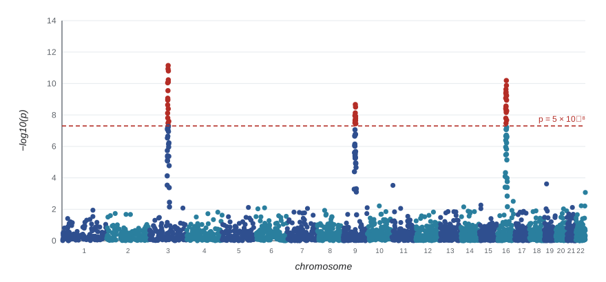
Because millions of tests are carried out, a p-value of 0.05 would yield tens of thousands of false positives. The conventional genome-wide significance threshold for studies of European-ancestry samples is p < 5 × 10⁻⁸. It corresponds to a Bonferroni correction for about one million independent tests, the approximate number of independent common variants in such genomes given their LD; populations with shorter LD, such as many African populations, have more independent variants and arguably need a stricter threshold. Results are displayed on a Manhattan plot, with −log₁₀(p) plotted against genomic position, where true associations appear as towers of correlated SNPs rising above the threshold line.
Confounding by population structure
The most serious pitfall in association studies is population stratification. If a sample combines groups that differ both in allele frequencies and in the average value of a trait, for reasons that may be entirely environmental, every SNP with a frequency difference between the groups will appear associated with the trait. A classic example is a study of type 2 diabetes in the Pima and Tohono O’odham peoples, where an apparent association with an immunoglobulin haplotype reflected differences in European admixture between participants, not a causal effect. Stratification inflates test statistics across the whole genome, which can be measured by the genomic inflation factor λ, the median observed chi-square statistic divided by its expected value under the null, 0.455. The standard remedies are to include the top principal components of the genotype matrix as covariates, or to fit linear mixed models that account for the genetic relatedness among all individuals.
import numpy as np
from scipy import stats
rng = np.random.default_rng(322)

n, m = 2000, 3000
grp = np.r_[np.zeros(n // 2), np.ones(n // 2)]               # two invented subpopulations
anc = rng.uniform(0.1, 0.9, m)
F = 0.05
p0 = rng.beta(anc * (1 - F) / F, (1 - anc) * (1 - F) / F)
p1 = rng.beta(anc * (1 - F) / F, (1 - anc) * (1 - F) / F)
P = np.where(grp[:, None] == 0, p0, p1)
G = rng.binomial(2, P).astype(float)

causal = rng.choice(m, 10, replace=False)
y = G[:, causal] @ rng.normal(0, 0.15, 10) + 0.5 * grp + rng.normal(0, 1, n)   # group effect is environmental

def scan(y, G, covars=None):
    X0 = np.ones((len(y), 1)) if covars is None else np.c_[np.ones(len(y)), covars]
    beta0 = np.linalg.lstsq(X0, y, rcond=None)[0]; r = y - X0 @ beta0
    Gr = G - X0 @ np.linalg.lstsq(X0, G, rcond=None)[0]       # residualize genotypes too
    b = (Gr * r[:, None]).sum(0) / (Gr**2).sum(0)
    resid = r[:, None] - Gr * b
    se = np.sqrt((resid**2).sum(0) / (len(y) - X0.shape[1] - 1) / (Gr**2).sum(0))
    chi2 = (b / se)**2
    return stats.chi2.sf(chi2, 1), np.median(chi2) / 0.455

Z = (G - G.mean(0)) / (G.std(0) + 1e-9)
pcs = np.linalg.svd(Z, full_matrices=False)[0][:, :2]
for label, cov in [("no correction", None), ("2 principal components", pcs)]:
    p, lam = scan(y, G, cov)
    print(f"{label:24s}: lambda = {lam:.2f}, SNPs with p < 1e-4 = {np.sum(p < 1e-4):3d}, "
f"of which causal = {np.sum(p[causal] < 1e-4)}")no correction : lambda = 8.71, SNPs with p < 1e-4 = 545, of which causal = 4 2 principal components : lambda = 1.06, SNPs with p < 1e-4 = 3, of which causal = 3
Without correction, the environmental difference between the two groups makes hundreds of non-causal SNPs appear associated, and λ is far above 1. Adding the first two principal components as covariates removes the inflation and leaves mainly the causal variants. Residual stratification along subtler axes of ancestry remains a concern in very large studies, which is why family-based designs comparing siblings, whose genotypes differ only by random segregation, have become an important check: associations that weaken sharply within families are likely to reflect stratification, assortative mating or indirect genetic effects of parents rather than direct effects.
What GWAS have found
Thousands of GWAS have identified hundreds of thousands of associations, and several general lessons have emerged. Most complex traits are extremely polygenic: a 2022 study of height in about 5.4 million people identified over 12,000 independent associated SNPs, which together captured most of the heritability attributable to common variants. Most associated variants lie outside protein-coding sequence, in regulatory regions, so identifying the causal variant and gene requires fine-mapping and functional work. Effect sizes are usually tiny, often a millimetre or two of height per allele. Effect sizes estimated in the discovery study tend to be exaggerated, a phenomenon called the winner’s curse, because variants that barely cross the threshold are more likely to have had overestimated effects by chance. And the SNPs reaching significance typically explain much less variance than twin studies suggest, the ‘missing heritability’, part of which is captured when all SNPs are analysed jointly (SNP heritability) and part of which may lie in rare variants or reflect biases in twin estimates.
| Approach | Population | Resolution | Strengths | Limitations |
|---|---|---|---|---|
| QTL mapping in crosses | F2, backcross or recombinant inbred lines | Tens of cM | Controlled environment; detects large-effect loci | Only parental differences; poor resolution |
| Multi-parent panels | Collaborative Cross, MAGIC lines | A few cM to sub-cM | More alleles, better resolution | Costly to build |
| GWAS | Natural populations | Tens of kb (depends on LD) | Many variants; high resolution | Stratification; small effects; needs huge samples |
| Family-based GWAS | Siblings or trios | As GWAS | Robust to stratification; isolates direct effects | Lower power per individual |
Polygenic scores and their portability
A polygenic score adds up an individual’s alleles at many variants, each weighted by its estimated effect from a GWAS. For some traits, polygenic scores now predict a meaningful fraction of variation in people similar to those in the discovery sample: scores for height explain roughly 40 per cent of its variance in people of European ancestry. In medicine they can help identify people at elevated risk of coronary artery disease or breast cancer, alongside conventional risk factors. In plant and animal breeding, the related method of genomic selection, which predicts breeding values from genome-wide markers, has transformed dairy cattle breeding since about 2009 by allowing young bulls to be evaluated from their DNA without waiting for daughters’ milk records.
The accuracy of a polygenic score falls as the genetic ancestry of the person being scored becomes more distant from that of the discovery sample. Alicia Martin and colleagues reported in 2019 that, for the scores then available, prediction accuracy was on average about two times lower in East Asian-ancestry and about four and a half times lower in African-ancestry individuals than in European-ancestry individuals. Later work by Yi Ding and colleagues in 2023 showed that accuracy declines continuously with genetic distance at the level of individuals, so that grouping people into discrete ancestry categories hides wide variation within them. The reasons are population genetic: allele frequencies differ, so variants common in one group may be rare in another; LD patterns differ, so a SNP that tags a causal variant well in one population may tag it poorly in another; and effects may interact with environments that differ among populations. Because most GWAS participants have been of European ancestry, these differences risk widening health disparities if scores are used clinically without care. Diversifying the people studied, through initiatives such as the All of Us Research Program in the United States and, in Canada, Indigenous-led projects such as Silent Genomes discussed in lesson 12, is the main remedy.
It is important to be clear about what polygenic scores do not show. Heritability within a population says nothing about the causes of average differences between populations, which can be entirely environmental. A polygenic score difference between groups, computed from GWAS effect sizes, can arise from residual stratification in the GWAS, from LD and frequency differences or from environmental confounding, and is not evidence of genetic differences in the trait. Genetic ancestry is continuous and describes where in the world a person’s ancestors lived; it is not a set of fixed biological types, and it is not the same as race, which is a social classification.
Common mistakes
MistakeTreating heritability as a fixed property of a trait.
InsteadV_A depends on allele frequencies and environments, so heritability is specific to a population and time.
MistakeAssuming a rare recessive allele of large effect explains much trait variance.
InsteadFew individuals are homozygous, so its contribution to variance is small.
MistakeIgnoring population structure in an association study.
InsteadInclude principal components or a mixed model, and check the genomic inflation factor.
MistakeTaking effect sizes from the discovery GWAS at face value.
InsteadThe winner’s curse inflates them; estimate effects in an independent replication sample.
MistakeInterpreting polygenic score differences between groups as genetic differences.
InsteadStratification, LD and environment can create such differences; heritability within groups does not explain differences between them.
Summary and key terms
- At one locus, V_A = 2pq[a + d(q − p)]² and V_D = (2pqd)²; both depend on allele frequency.
- Fisher’s infinitesimal model explains normal trait distributions and the persistence of additive variance.
- QTL mapping in crosses finds large-effect loci but localizes them only to broad regions.
- GWAS test millions of variants; p < 5 × 10⁻⁸ is the conventional genome-wide threshold, and stratification must be corrected.
- Most traits are highly polygenic, most associations are regulatory, and discovery effect sizes are inflated by the winner’s curse.
- Polygenic score accuracy declines continuously with genetic distance from the discovery sample; scores do not explain group differences.
- additive genetic variance
- The part of genetic variance due to average effects of alleles, which determines resemblance between parents and offspring.
- dominance variance
- Genetic variance due to interactions between alleles at the same locus.
- average effect
- α = a + d(q − p), the mean change in trait value from substituting one allele for another.
- infinitesimal model
- Fisher’s model of a trait influenced by very many loci of tiny effect.
- QTL
- A quantitative trait locus: a chromosome region containing variants that affect a quantitative trait.
- LOD score
- The base-10 logarithm of the likelihood ratio for a QTL at a position versus no QTL.
- genome-wide significance
- The threshold p < 5 × 10⁻⁸ used to declare associations in GWAS.
- population stratification
- Confounding of association results by differences in ancestry and trait means among subgroups.
- winner’s curse
- The overestimation of effect sizes for associations discovered at a stringent threshold.
- polygenic score
- A weighted sum of an individual’s alleles at many variants, used to predict a trait.
Practice problems
Work each problem on paper first, then reveal the answer to check.
A locus has a = 1, d = 0 and p = 0.3. What is V_A?
Show answer
2 × 0.3 × 0.7 × 1 = 0.42.
With a = 1, d = 0.5 and p = 0.3, what is α?
Show answer
1 + 0.5 × (0.7 − 0.3) = 1.2.
For the same locus, what are V_A and V_D?
Show answer
V_A = 0.42 × 1.44 ≈ 0.605; V_D = (0.42 × 0.5)² ≈ 0.044.
Why does the threshold 5 × 10⁻⁸ correspond to about one million tests?
Show answer
0.05/1,000,000 = 5 × 10⁻⁸ (Bonferroni).
A GWAS has a median chi-square of 0.60. What is λ, and what does it suggest?
Show answer
λ = 0.60/0.455 ≈ 1.32, suggesting inflation from stratification or relatedness, or extreme polygenicity.
Why is QTL resolution in an F2 population poor?
Show answer
Only one or two rounds of recombination, so LD extends over tens of centimorgans.
What is the winner’s curse?
Show answer
Overestimation of effect sizes for variants that pass a stringent threshold in the discovery sample.
Give two population-genetic reasons why polygenic scores transfer poorly across ancestries.
Show answer
Differences in allele frequencies and in LD between tag SNPs and causal variants.
How do sibling comparisons help in GWAS?
Show answer
Sibling genotype differences are random, so they are not confounded by population stratification.
Does high heritability of a trait within two populations imply that a difference in means between them is genetic?
Show answer
No; heritability within groups says nothing about the causes of differences between them.
Lesson quiz · 5 questions
Score 60% or more to complete this lesson.
Create a free account to save your progress, take quizzes and earn a certificate.