
BIOL-322 · Lesson 5 of 12 · 26 min
The interplay of drift, selection and mutation
Lessons 3 and 4 treated selection and drift separately: selection as a deterministic push in one direction, drift as random wandering with no direction at all. Real populations experience both at once, and new variation is constantly supplied by mutation. The outcome depends on their relative strengths, and one compound parameter, the product of effective size and selection coefficient, decides which force wins. This lesson develops Kimura’s formula for the probability that a selected allele is fixed, explains the nearly neutral zone in which drift overrides weak selection, works out how long selected alleles take to fix, describes the equilibrium between mutation and drift, and shows why small populations accumulate harmful mutations, a central concern of conservation genomics.
Kimura’s fixation probability
In 1962 Motoo Kimura used the diffusion approximation to find the probability that an allele with additive selective advantage s, currently at frequency p, will eventually be fixed in a population with effective size N_e:
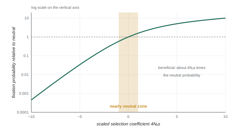
Here s is the advantage of each copy of the allele, so the heterozygote has fitness 1 + s and the favoured homozygote 1 + 2s; note that this differs by a factor of 2 from the convention used for additive selection in lesson 3. The formula behaves sensibly at its limits. As s approaches zero it reduces to u(p) = p, the neutral result. For a single new mutation in a diploid population of census size N, p = 1/(2N). When 4N_e s is large and positive, the denominator approaches 1 and u ≈ 1 − e^(−2s N_e/N), which for small s is about 2s N_e/N, or simply 2s when N_e = N. This is Haldane’s classic result: even a mutation with a 1 per cent advantage is lost about 98 times out of 100, because while it is present in only a few copies, its fate is governed by chance. Beneficial mutations must survive this early stochastic phase before selection takes control.
When s is negative, u is not zero. A deleterious mutation can still be fixed by drift, but its probability falls off exponentially once |4N_e s| exceeds about 1. With N_e = 10,000 and s = −0.001 (4N_e s = −40), the fixation probability of a new mutation is about 10⁻²¹, effectively zero. With N_e = 100 and the same s (4N_e s = −0.4), it is about 0.0041, close to the neutral 0.005. The same mutation is effectively neutral in a small population and strongly selected against in a large one.
import numpy as np
import warnings; warnings.filterwarnings("ignore")
rng = np.random.default_rng(322)

def kimura(p, s, Ne):
    if s == 0:
        return p
    return (1 - np.exp(-4*Ne*s*p)) / (1 - np.exp(-4*Ne*s))

def simulate(N, s, reps=40000):
    # Wright-Fisher with additive selection, starting from one copy
    p = np.full(reps, 1 / (2*N))
    alive = np.ones(reps, bool)
    while alive.any():
        q = p[alive]
        q = q * (1 + s) / (1 + s*q)            # haploid-style selection on allele copies
        p[alive] = rng.binomial(2*N, q) / (2*N)
        alive = (p > 0) & (p < 1)
    return np.mean(p == 1)

N = 50
for s in (-0.01, 0.0, 0.01, 0.05):
    sim = simulate(N, s)
    print(f"s = {s:+.2f} (4Ns = {4*N*s:+5.1f}): simulated u = {sim:.4f}, "
f"Kimura u = {kimura(1/(2*N), s, N):.4f}, neutral = {1/(2*N):.4f}")s = -0.01 (4Ns = -2.0): simulated u = 0.0034, Kimura u = 0.0032, neutral = 0.0100 s = +0.00 (4Ns = +0.0): simulated u = 0.0099, Kimura u = 0.0100, neutral = 0.0100 s = +0.01 (4Ns = +2.0): simulated u = 0.0232, Kimura u = 0.0229, neutral = 0.0100 s = +0.05 (4Ns = +10.0): simulated u = 0.0934, Kimura u = 0.0952, neutral = 0.0100
The simulated fixation probabilities agree with Kimura’s formula across beneficial, neutral and deleterious mutations. Here the selection step multiplies each allele copy’s weight by 1 + s, which is equivalent to additive selection with coefficient s per copy for small s.
The nearly neutral zone
The scaled selection coefficient S = 4N_e s determines whether selection or drift dominates. When |S| is much greater than 1, selection rules: beneficial mutations fix far more often than neutral ones and deleterious ones almost never fix. When |S| is much less than 1, mutations behave as if neutral. Between these lies a zone, roughly |S| between 0.1 and 10, where both forces matter. Tomoko Ohta’s nearly neutral theory, developed from 1973, proposed that many mutations fall in this zone, especially slightly deleterious amino acid changes. Its key prediction is that the rate of molecular evolution should depend on population size: species with small N_e should fix more slightly deleterious mutations, so their proteins should evolve faster at non-synonymous sites relative to synonymous sites.
Comparative genomic data broadly support this prediction. Species with small long-term effective sizes, such as large mammals, tend to have higher ratios of non-synonymous to synonymous diversity and divergence than species with very large effective sizes, such as Drosophila or many bacteria. Michael Lynch extended the argument into the drift-barrier hypothesis, which proposes that selection can refine a trait only until the remaining improvements are so small that drift overwhelms them. Because the barrier is set by N_e, organisms with small populations should tolerate more genomic clutter, such as introns and transposable elements, and should even have higher mutation rates, because selection to improve replication fidelity runs out of power sooner. Lynch’s data show that mutation rates per nucleotide are indeed lower in organisms with larger effective sizes.
| Effective size | Mutation with s = −0.0001 | Mutation with s = −0.001 | Mutation with s = −0.01 |
|---|---|---|---|
| 100 | Effectively neutral (4N_e s = −0.04) | Nearly neutral (−0.4) | Selected against (−4) |
| 10,000 | Nearly neutral (−4) | Selected against (−40) | Strongly selected against (−400) |
| 1,000,000 | Selected against (−400) | Strongly selected against | Strongly selected against |
How long does a selected allele take to fix?
For an allele that does go to fixation, the time required depends on both s and N. Selection shortens the journey compared with drift, but the approximate time for a new beneficial mutation that escapes early loss is about (2/s) ln(2N) generations for an additive allele, compared with 4N_e for a neutral one. With N = 10,000 and s = 0.01, that is about 2,000 generations rather than 40,000. Fixation times matter because, as lesson 9 explains, a rapid sweep drags linked neutral variation along with it and leaves a signature in the surrounding genome; the faster the sweep, the wider the region of reduced diversity.
Worked problem
Fate of a beneficial mutation
A new mutation arises in a population with N = N_e = 5,000 and gives an additive advantage s = 0.004. What is its probability of fixation, and roughly how long will a successful sweep take?
Show solution
- Scaled selection: 4N_e s = 4 × 5,000 × 0.004 = 80, so selection dominates once the allele is common.
- Fixation probability ≈ 2s = 0.008 (Kimura’s formula gives 1 − e^(−0.008) ≈ 0.0080).
- Neutral fixation probability would be 1/(2N) = 0.0001, so selection makes fixation 80 times more likely.
- Time to fixation if successful ≈ (2/s) ln(2N) = 500 × ln(10,000) ≈ 500 × 9.21 ≈ 4,600 generations.
Answer: About 0.8 per cent of such mutations fix, and each successful one takes roughly 4,600 generations, compared with about 20,000 generations for a neutral mutation that happens to fix.
Mutation and drift in balance
Drift removes variation at a rate of 1/(2N_e) per generation; mutation adds it. Eventually the two balance. Under the infinite-alleles model, in which every mutation creates a new allele never seen before, the equilibrium expected heterozygosity depends only on the population mutation rate θ = 4N_eμ, where μ is the mutation rate per locus per generation:
A locus with μ = 10⁻⁴, typical of a microsatellite, in a population with N_e = 5,000 has θ = 2 and an expected heterozygosity of about 0.67. The same locus in a population of 50 has θ = 0.02 and H of about 0.02. This dependence on θ, not on N_e or μ separately, is a general feature of neutral theory: neutral diversity can never tell us N_e or μ on its own, only their product. To separate them, we need an independent estimate of the mutation rate.
For microsatellites, the stepwise mutation model is more realistic, because a mutation usually adds or removes a single repeat unit and so can recreate an existing allele. The equilibrium heterozygosity under that model is 1 − 1/√(1 + 2θ), which is lower than under the infinite-alleles model for the same θ because new mutations are often identical to existing alleles. Warren Ewens derived the full distribution of allele counts under the infinite-alleles model in 1972. The Ewens sampling formula shows that the expected number of distinct alleles in a sample of n gene copies is Σθ/(θ + i) for i from 0 to n − 1, which grows only logarithmically with sample size, one reason why allelic richness must be standardized.
import numpy as np
rng = np.random.default_rng(3225)

def infinite_alleles(N, mu, gens):
    # 2N gene copies; each new mutation creates a brand new allele label
    pop = np.zeros(2*N, dtype=np.int64); next_label = 1
    for _ in range(gens):
        pop = rng.choice(pop, size=2*N, replace=True)          # drift
        m = rng.random(2*N) < mu                                # mutation
        k = m.sum()
        pop[m] = np.arange(next_label, next_label + k); next_label += k
    _, counts = np.unique(pop, return_counts=True)
    f = counts / (2*N)
    return 1 - np.sum(f**2), len(counts)

N, mu = 250, 0.001
theta = 4 * N * mu
H_runs = [infinite_alleles(N, mu, 4000)[0] for _ in range(20)]
print(f"theta = {theta:.1f}")
print(f"simulated mean H = {np.mean(H_runs):.3f} (sd among runs {np.std(H_runs):.3f})")
print(f"theory theta/(1+theta) = {theta/(1+theta):.3f}")
print(f"stepwise model would give {1 - 1/np.sqrt(1 + 2*theta):.3f}")theta = 1.0 simulated mean H = 0.460 (sd among runs 0.196) theory theta/(1+theta) = 0.500 stepwise model would give 0.423
The mean of the replicate simulations sits close to θ/(1 + θ), but individual runs vary widely around it. That variation is not a flaw in the simulation; it is the real evolutionary variance of drift, and it is why the heterozygosity of a single locus is a poor estimate of θ. Averages across many independent loci are needed.
Mutation rates
The neutral mutation rate is the ultimate source of all variation, and estimates have improved dramatically with sequencing of parents and offspring. In humans, whole-genome sequencing of families gives a germline rate of roughly 1.2 × 10⁻⁸ per base pair per generation, or about 60 to 70 new single-nucleotide mutations in each child’s genome. Most of these come from the father, and their number rises with paternal age, by roughly one to two additional mutations per year, because sperm-producing cells keep dividing throughout adult life. Combined with π ≈ 0.001 and π ≈ 4N_eμ for a diploid, this mutation rate implies a long-term human effective size of about 0.001/(4 × 1.2 × 10⁻⁸) ≈ 20,000, tiny compared with the eight billion people alive today and a reminder that diversity records the deep past.
Small populations accumulate harmful mutations
Combining these results explains a core concern of conservation genetics. In small populations, more slightly deleterious mutations fall into the nearly neutral zone, so they drift to higher frequency and sometimes fix; this is drift load. At the same time, inbreeding exposes recessive deleterious alleles in homozygotes, which causes inbreeding depression but can also purge strongly deleterious recessive alleles, because selection can finally act on them. Purging is efficient for lethal and severely harmful recessives but much less so for mildly harmful mutations, which accumulate. Genomic studies of island foxes, Isle Royale wolves, mountain gorillas and the extinct woolly mammoths of Wrangel Island have documented these processes, with some populations showing fewer highly damaging variants but more homozygous mildly damaging ones than their larger relatives.
In asexual populations or non-recombining chromosomes, a related process called Muller’s ratchet operates: once the class of genomes carrying the fewest harmful mutations is lost by drift, it cannot be recreated without back mutation or recombination, so the load can only ratchet upward. This helps explain the degeneration of Y chromosomes and of the genomes of endosymbiotic bacteria, and it is one of the arguments for the advantage of sexual reproduction.
Common mistakes
MistakeAssuming a beneficial mutation will fix because selection favours it.
InsteadA new beneficial mutation is usually lost by drift; its fixation probability is only about 2s.
MistakeTreating a selection coefficient as meaningful on its own.
InsteadWhat matters is 4N_e s: the same s can be neutral in a small population and strongly selected in a large one.
MistakeInferring N_e from diversity without an independent mutation rate.
InsteadNeutral diversity depends on θ = 4N_eμ; N_e and μ cannot be separated from diversity alone.
MistakeExpecting purging to remove all harmful variation from inbred populations.
InsteadPurging works mainly on strongly deleterious recessives; mildly deleterious mutations accumulate as drift load.
MistakeUsing the infinite-alleles formula for microsatellites.
InsteadStepwise mutation recreates existing alleles, so equilibrium heterozygosity is lower: 1 − 1/√(1 + 2θ).
Summary and key terms
- Kimura’s formula u(p) = (1 − e^(−4N_e s p))/(1 − e^(−4N_e s)) gives fixation probabilities under selection and drift.
- A new beneficial mutation fixes with probability about 2s; most are lost while rare.
- The scaled coefficient 4N_e s decides whether drift or selection dominates; |4N_e s| below about 1 is nearly neutral.
- Small populations fix more slightly deleterious mutations, which underlies the nearly neutral theory and the drift-barrier hypothesis.
- Mutation–drift balance under infinite alleles gives H = θ/(1 + θ), with θ = 4N_eμ.
- Human germline mutation rates are about 1.2 × 10⁻⁸ per base per generation, implying a long-term N_e of about 20,000.
- fixation probability
- The probability that an allele eventually reaches frequency 1.
- scaled selection coefficient
- 4N_e s, which measures the strength of selection relative to drift.
- nearly neutral theory
- Ohta’s theory that many mutations are slightly deleterious and behave as neutral in small populations.
- drift-barrier hypothesis
- Lynch’s idea that selection can refine traits only until improvements fall below the power of drift.
- population mutation rate
- θ = 4N_eμ, the parameter that governs neutral diversity in diploids.
- infinite-alleles model
- A mutation model in which each mutation creates a new, unique allele.
- stepwise mutation model
- A model in which mutations add or remove one repeat unit, suitable for microsatellites.
- Ewens sampling formula
- The distribution of allele counts in a sample under neutral infinite-alleles evolution.
- drift load
- Reduced fitness caused by fixation of deleterious alleles through drift in small populations.
- Muller’s ratchet
- The irreversible accumulation of harmful mutations in populations without recombination.
Practice problems
Work each problem on paper first, then reveal the answer to check.
What is the approximate fixation probability of a new mutation with s = 0.03 when N_e = N?
Show answer
About 2s = 0.06.
Calculate 4N_e s for N_e = 500 and s = −0.0002. How will the mutation behave?
Show answer
−0.4: nearly neutral; it fixes almost as often as a neutral mutation.
If N_e is half of N, what is the fixation probability of a mutation with s = 0.02?
Show answer
About 2s N_e/N = 0.02.
Use Kimura’s formula: what is u(0.5) for a neutral allele?
Show answer
0.5.
About how long does a sweep take if s = 0.02 and N = 50,000?
Show answer
(2/0.02) ln(100,000) ≈ 100 × 11.5 ≈ 1,150 generations.
What is H_eq under infinite alleles if θ = 0.5?
Show answer
0.5/1.5 ≈ 0.33.
What is H_eq under stepwise mutation if θ = 4?
Show answer
1 − 1/√9 = 1 − 1/3 ≈ 0.67.
What θ is implied by π = 0.0016 in a diploid species, and what N_e if μ = 2 × 10⁻⁸?
Show answer
θ ≈ 0.0016 per site; N_e = 0.0016/(4 × 2 × 10⁻⁸) = 20,000.
Why does purging remove lethal recessives more effectively than mildly harmful ones?
Show answer
Lethals are strongly selected once exposed in homozygotes; mild mutations fall in the nearly neutral zone in small populations.
What does Muller’s ratchet predict for a non-recombining chromosome?
Show answer
Irreversible accumulation of harmful mutations as the least-loaded class is lost by drift.
Lesson quiz · 5 questions
Score 60% or more to complete this lesson.
Create a free account to save your progress, take quizzes and earn a certificate.