
BIOL-322 · Lesson 3 of 12 · 29 min
Natural selection: single-locus models and equilibria
Natural selection is the only evolutionary force that systematically adapts organisms to their environments. BIOL-321 described the modes of selection, directional, stabilizing, disruptive and frequency-dependent, and showed how dominance affects the speed of response. This lesson builds the single-locus theory more carefully. We write down the general recursion for a diploid locus, find its equilibria, decide which equilibria are stable, work out how long selection takes, and calculate how much harmful variation persists when selection is balanced against recurrent mutation. These results are the building blocks for everything that follows, from fixation probabilities in lesson 5 to the detection of selection in genomes in lesson 10.
Fitness and the general recursion
Consider a locus with alleles A1 and A2 at frequencies p and q. Assign the three genotypes relative fitnesses w11, w12 and w22, where fitness is the expected contribution of an individual to the next generation’s gene pool relative to other genotypes. If selection acts on survival from zygote to adult and adults then mate at random, the genotype frequencies after selection are proportional to p²w11, 2pqw12 and q²w22. Their sum is the mean fitness:
The new frequency of A1 is p' = (p²w11 + pqw12)/w̄, and the change over one generation simplifies to a form that reveals the structure of selection:
Three features of this formula are worth noticing. First, the factor pq means that selection is slow when either allele is rare: there is little variation for it to act on. Second, the term in square brackets is the difference between the average fitness of A1 and A2 alleles, called the average excess; when it is positive, A1 increases. Third, Sewall Wright showed that the same expression can be written as Δp = (pq/2w̄) dw̄/dp, so that, for constant fitnesses, selection moves p uphill on a curve of mean fitness. This is the original adaptive landscape, and in this simple case selection always increases w̄, a single-locus version of Fisher’s fundamental theorem.
It is convenient to write fitnesses in terms of a selection coefficient s and a dominance coefficient h, with w11 = 1, w12 = 1 − hs and w22 = 1 − s. When h = 0, A2 is fully recessive in its effect on fitness; when h = 1, it is dominant; when h = 0.5, effects are additive. Values of h below 0 or above 1 describe overdominance and underdominance, which we treat separately because they give interior equilibria.
| Fitness pattern | w11 : w12 : w22 | Equilibria | Outcome |
|---|---|---|---|
| Directional, additive | 1 : 1 − s/2 : 1 − s | p = 0 (unstable), p = 1 (stable) | A1 goes to fixation from any starting frequency |
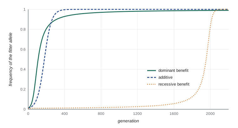
| Directional, A1 dominant | 1 : 1 : 1 − s | p = 0 (unstable), p = 1 (stable) | Fast spread at first, very slow final elimination of A2 |
| Directional, A1 recessive | 1 : 1 − s : 1 − s | p = 0 (unstable), p = 1 (stable) | Very slow start, fast finish |
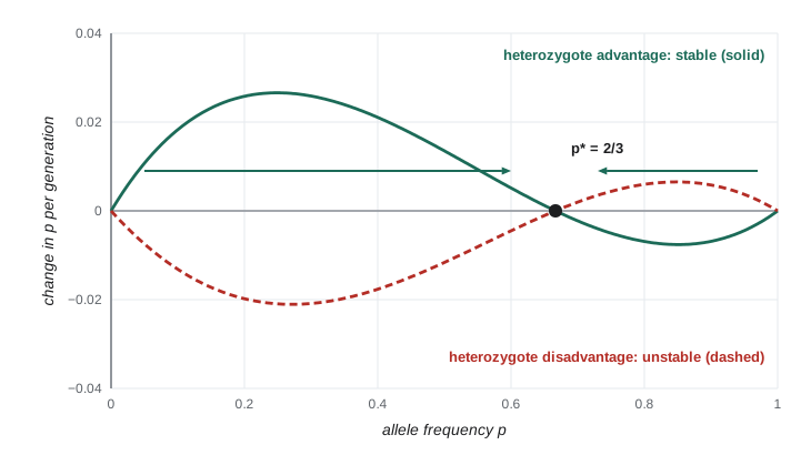
| Overdominance (heterozygote advantage) | 1 − s : 1 : 1 − t | Interior p* = t/(s + t) stable | Both alleles maintained |
| Underdominance (heterozygote disadvantage) | 1 + s : 1 : 1 + t | Interior p* = t/(s + t) unstable | Fixation of whichever allele starts above threshold |
Equilibria and their stability
An equilibrium is a frequency at which Δp = 0. From the general formula, p = 0 and p = 1 are always equilibria, because selection cannot act on an allele that is absent. An interior equilibrium exists when the average excesses of the two alleles are equal, which requires the heterozygote to be either fitter or less fit than both homozygotes. Writing w11 = 1 − s, w12 = 1 and w22 = 1 − t for heterozygote advantage, the interior equilibrium is:
To test stability, ask what happens after a small displacement. With heterozygote advantage, if p rises slightly above p*, more A1A1 homozygotes are produced and they are less fit, so p falls back; p* is stable. With heterozygote disadvantage, the same displacement is amplified, because heterozygotes are now the least fit class and the more common allele is favoured; p* is unstable and acts as a threshold. Underdominance helps explain why chromosomal rearrangements that reduce fertility in heterozygotes rarely spread, and it is the principle behind some proposed gene-drive and Wolbachia strategies for insect control, which must be released above a threshold frequency to take over.
Worked problem
Sickle-cell hemoglobin as balanced polymorphism
In a malaria-endemic region, suppose (illustratively) that relative fitnesses are 0.88 for HbA/HbA (malaria mortality), 1 for HbA/HbS and 0.20 for HbS/HbS (sickle-cell disease without modern care). What equilibrium frequency of HbS is expected?
Show solution
- Write fitnesses as 1 − s for AA and 1 − t for SS: s = 0.12 and t = 0.80.
- The equilibrium frequency of A is p* = t/(s + t) = 0.80/0.92 ≈ 0.870.
- So the equilibrium frequency of HbS is q* = s/(s + t) = 0.12/0.92 ≈ 0.13.
- At that frequency about 2 × 0.87 × 0.13 ≈ 23 per cent of people are carriers and about 1.7 per cent have sickle-cell disease.
Answer: About 0.13, close to frequencies observed in parts of West and Central Africa; the fitness values here are illustrative, and real values vary with malaria intensity and access to treatment.
Heterozygote advantage was once thought to explain much of the variation discovered by electrophoresis, but clear cases are few. The sickle-cell allele is the best documented; others involve glucose-6-phosphate dehydrogenase deficiency and thalassemias, also in relation to malaria. Balanced polymorphism does have a cost, the segregation load: because heterozygotes cannot breed true, every generation produces less fit homozygotes. Lewontin and others argued that if thousands of loci were maintained this way, the combined load would be impossibly large, one of the arguments that pushed the field toward neutral explanations.
How fast does selection work?
For an allele with an additive advantage s, and while s is small, the frequency follows a logistic curve, and the time to go from frequency p_0 to p_t is approximately:
(The factor 2 appears because, with fitnesses 1, 1 − s/2 and 1 − s, each copy of the favoured allele raises fitness by s/2.) Going from 1 per cent to 99 per cent therefore takes about (2/s) × ln(9,801) ≈ 18.4/s generations: about 1,840 generations for s = 0.01, or 184 for s = 0.1. Dominance changes the shape of the trajectory dramatically. A favoured dominant allele spreads quickly at first, because heterozygotes already enjoy the full advantage, but the last few recessive copies of the disfavoured allele hide in heterozygotes and are removed very slowly. A favoured recessive allele is the mirror image: when it is rare it occurs almost only in heterozygotes, where it has no effect, so it starts extremely slowly. This asymmetry is known as Haldane’s sieve: new beneficial mutations that are at least partly dominant are much more likely to contribute to adaptation, both because they spread faster and, as lesson 5 shows, because they are less likely to be lost by drift when rare.
import numpy as np

def trajectory(p0, s, h, gens=4000):
    # A1 is the fitter allele; fitnesses 1, 1 - h*s, 1 - s for A1A1, A1A2, A2A2
    p = p0; out = [p]
    w11, w12, w22 = 1.0, 1 - h*s, 1 - s
    for _ in range(gens):
        q = 1 - p
        wbar = p*p*w11 + 2*p*q*w12 + q*q*w22
        p = (p*p*w11 + p*q*w12) / wbar
        out.append(p)
    return np.array(out)

s = 0.05
for name, h in [("A1 dominant (h = 0)", 0.0), ("additive (h = 0.5)", 0.5), ("A1 recessive (h = 1)", 1.0)]:
    tr = trajectory(0.01, s, h)
    t50 = np.argmax(tr >= 0.5); t99 = np.argmax(tr >= 0.99)
    print(f"{name:22s}: reaches 0.5 at gen {t50:4d}, 0.99 at gen {t99:4d}")

approx = (2 / s) * np.log(0.99 * 0.99 / (0.01 * 0.01))
print(f"logistic approximation for additive case, 0.01 to 0.99: {approx:.0f} generations")A1 dominant (h = 0) : reaches 0.5 at gen 110, 0.99 at gen 2157 additive (h = 0.5) : reaches 0.5 at gen 178, 0.99 at gen 359 A1 recessive (h = 1) : reaches 0.5 at gen 1954, 0.99 at gen 2063 logistic approximation for additive case, 0.01 to 0.99: 368 generations
In this code, h measures how much of the disadvantage of A2A2 is expressed in heterozygotes, so h = 0 makes the heterozygote as fit as A1A1 (the benefit of A1 is dominant) and h = 1 makes it as unfit as A2A2 (the benefit is recessive). Reading the printed times, the additive case is close to the logistic approximation; the dominant case reaches 50 per cent fastest but then needs well over a thousand more generations to approach fixation; and the recessive case barely moves for most of two thousand generations before sweeping rapidly to fixation.
Mutation–selection balance
Harmful mutations are constantly produced and constantly removed. At equilibrium, the rate at which new copies of a deleterious allele arise by mutation equals the rate at which selection eliminates them. Suppose mutation converts the normal allele to a deleterious one at rate μ per generation and the deleterious homozygote has fitness 1 − s. For a fully recessive allele, selection acts only on homozygotes, which occur at frequency q², and the equilibrium is:
Even slight dominance changes the picture enormously. Take μ = 10⁻⁵ and a lethal allele (s = 1). If it is fully recessive, q̂ is about 0.0032, so about one person in 160 is a carrier. If it reduces heterozygote fitness by just 2 per cent (h = 0.02), q̂ falls to 0.0005, more than six times lower, because selection now acts on the far more numerous heterozygotes. This is why many severe recessive disease alleles persist at low but stable frequencies, and why changes in mating patterns, such as an increase in consanguineous marriage, change the incidence of recessive disease far more than they change allele frequencies.
import numpy as np

def equilibrium(mu, s, h, gens=200000):
    q = 0.0
    for _ in range(gens):
        q = q + mu * (1 - q)                       # mutation A -> a
        p = 1 - q
        wbar = p*p + 2*p*q*(1 - h*s) + q*q*(1 - s)
        q = (p*q*(1 - h*s) + q*q*(1 - s)) / wbar     # selection
    return q

mu, s = 1e-5, 1.0
for h in (0.0, 0.02, 0.1):
    q = equilibrium(mu, s, h)
    approx = np.sqrt(mu / s) if h == 0 else mu / (h * s)
    print(f"h = {h:4.2f}: simulated q = {q:.5f}, approximation = {approx:.5f}, "
f"carriers per 10,000 = {2*q*(1-q)*1e4:.1f}")h = 0.00: simulated q = 0.00315, approximation = 0.00316, carriers per 10,000 = 62.8 h = 0.02: simulated q = 0.00048, approximation = 0.00050, carriers per 10,000 = 9.6 h = 0.10: simulated q = 0.00009, approximation = 0.00010, carriers per 10,000 = 1.8
The simulated equilibria match the approximations. Summed over the whole genome, the reduction in mean fitness caused by deleterious mutations, the mutation load, depends only on the total mutation rate and not on how harmful each mutation is: at equilibrium, every harmful mutation eventually causes one genetic death, whatever its effect. For partly dominant mutations, the load per locus is about 2μ; for fully recessive ones, about μ. With a genomic deleterious mutation rate of perhaps one or more per generation in humans, these simple calculations raised questions about how populations tolerate such loads, questions answered in part by synergistic interactions among mutations and by soft selection.
Beyond viability: other forms of selection
The models so far assume constant fitnesses acting on survival. Several important extensions keep the same algebra but change the biology. With fertility selection, fitness depends on the mating pair, not the individual, and equilibria can be more complex. With selection that differs between the sexes, an allele favoured in males and disfavoured in females can be maintained, a source of sexual conflict. With selection that varies over time, the long-run outcome depends on the geometric mean of fitnesses across generations, which favours genotypes that do consistently well over those that do brilliantly in some years and badly in others. With selection that varies in space, combined with migration, polymorphism can be maintained if migration is weak relative to selection, a theme lesson 8 returns to with clines.
Frequency-dependent selection, introduced in BIOL-321, also yields stable interior equilibria. Rare-allele advantage is common for self-incompatibility alleles in plants, which can number in the dozens at one locus, and for genes of the major histocompatibility complex, where rare variants may help hosts recognize pathogens that have adapted to common variants. The genetic signatures of these forms of balancing selection, including unusually old alleles and excess intermediate-frequency variation, are among the patterns lesson 10 teaches you to look for.
Worked problem
Time for a resistance allele to spread
An insecticide is applied every year to a pest with one generation per year. A resistance allele starts at frequency 0.001, is additive and has s = 0.2 in treated fields. Roughly how many years until it reaches 50 per cent?
Show solution
- Use t ≈ (2/s) ln[p_t(1 − p_0)/(p_0(1 − p_t))].
- p_0 = 0.001, p_t = 0.5: the ratio is (0.5 × 0.999)/(0.001 × 0.5) = 999.
- ln(999) ≈ 6.91; 2/s = 10.
- t ≈ 69 generations, so about 69 years with one generation per year.
- With several generations per year, or s near 1 as for some resistance alleles under heavy spraying, the time shrinks to a few years.
Answer: About 69 generations; refuges of untreated plants slow the process by reducing s averaged across the landscape and by keeping resistance alleles rare and mostly in heterozygotes, where they may be functionally recessive.
Common mistakes
MistakeThinking that a favoured dominant allele reaches fixation fastest.
InsteadIt reaches intermediate frequency fastest, but the last disfavoured recessive copies hide in heterozygotes and disappear very slowly.
MistakeTreating every interior equilibrium as stable.
InsteadCheck the sign of Δp on either side. Heterozygote advantage gives a stable equilibrium; heterozygote disadvantage gives an unstable threshold.
MistakeUsing √(μ/s) for a deleterious allele with any heterozygous effect.
InsteadUse μ/(hs) when h is not close to zero; even h = 0.02 changes the equilibrium several-fold.
MistakeAssuming that selection always maximizes mean fitness.
InsteadWith constant fitnesses at one locus it does, but frequency dependence, sex differences and multi-locus interactions can break this rule.
MistakeExpecting heterozygote advantage to explain most protein variation.
InsteadSegregation load makes widespread overdominance implausible; few cases are well documented.
Summary and key terms
- With genotype fitnesses w11, w12 and w22, Δp = pq[p(w11 − w12) + q(w12 − w22)]/w̄, which is slow when either allele is rare.
- Under constant fitnesses, selection moves p uphill on the curve of mean fitness.
- Heterozygote advantage gives a stable interior equilibrium p* = t/(s + t); heterozygote disadvantage gives an unstable threshold.
- An additive allele with advantage s takes about 18.4/s generations to go from 1 to 99 per cent; dominance strongly changes the trajectory.
- Mutation–selection balance gives q̂ ≈ √(μ/s) for recessive and μ/(hs) for partly dominant deleterious alleles.
- Selection that varies in time, space or between the sexes, and frequency-dependent selection, can maintain polymorphism.
- relative fitness
- The expected reproductive contribution of a genotype, scaled relative to a reference genotype.
- mean fitness
- The average fitness of all genotypes in the population, weighted by their frequencies.
- dominance coefficient
- h, the fraction of the homozygote’s fitness effect expressed in the heterozygote.
- overdominance
- Heterozygote advantage: the heterozygote is fitter than both homozygotes.
- underdominance
- Heterozygote disadvantage: the heterozygote is less fit than both homozygotes.
- stable equilibrium
- A frequency to which the population returns after a small displacement.
- Haldane’s sieve
- The bias toward dominant beneficial mutations contributing to adaptation.
- mutation–selection balance
- The equilibrium at which new deleterious mutations are removed by selection as fast as they arise.
- segregation load
- The reduction in mean fitness caused by producing less fit homozygotes at a balanced polymorphism.
- mutation load
- The reduction in mean fitness caused by recurrent deleterious mutation.
Practice problems
Work each problem on paper first, then reveal the answer to check.
With w11 = 1, w12 = 0.9 and w22 = 0.8 and p = 0.5, what is w̄?
Show answer
0.25 + 0.45 + 0.20 = 0.90.
For the same values, what is Δp?
Show answer
pq[p(0.1) + q(0.1)]/w̄ = 0.25 × 0.1/0.9 ≈ 0.028.
Fitnesses are 0.7, 1 and 0.9 for A1A1, A1A2 and A2A2. What is the equilibrium frequency of A1?
Show answer
s = 0.3, t = 0.1, so p* = 0.1/0.4 = 0.25.
Is that equilibrium stable?
Show answer
Yes, because the heterozygote is fittest.
If fitnesses are 1.2, 1 and 1.1, what happens to a population starting at p = 0.2?
Show answer
The threshold is p* = 0.1/0.3 ≈ 0.33; starting below it, A1 is lost and A2 fixes.
About how many generations does an additive allele with s = 0.02 take to go from 1 to 99 per cent?
Show answer
18.4/0.02 ≈ 920 generations.
A recessive lethal arises at μ = 4 × 10⁻⁶. What is its equilibrium frequency?
Show answer
√(4 × 10⁻⁶) = 0.002.
The same allele has h = 0.05. What is the equilibrium frequency now?
Show answer
μ/(hs) = 4 × 10⁻⁶/0.05 = 8 × 10⁻⁵.
Why does a rare favoured recessive allele spread so slowly at first?
Show answer
It occurs almost entirely in heterozygotes, where it has no effect on fitness.
What does the geometric mean fitness explain when fitness fluctuates over time?
Show answer
Genotypes with consistently good fitness can outcompete those with a higher arithmetic mean but more variable fitness.
Lesson quiz · 5 questions
Score 60% or more to complete this lesson.
Create a free account to save your progress, take quizzes and earn a certificate.