
BIOL-322 · Lesson 7 of 12 · 26 min
Population structure and F-statistics
Few species form a single randomly mating population. Individuals mate mostly with neighbours, populations are separated by mountains, rivers or stretches of ocean, and dispersal is limited. Under these conditions drift acts independently in each local population, allele frequencies diverge, and the species becomes genetically structured. Structure matters in almost every application of population genetics. It defines management units in conservation, it must be corrected for in forensic match probabilities, and if ignored it creates false associations in genome-wide studies. This lesson develops Sewall Wright’s F-statistics, the standard framework for describing structure, explains the Wahlund effect, compares estimators of F_ST, connects F_ST to coalescent times and the island model, and addresses common misreadings of structure in human populations.
The Wahlund effect
Suppose a sample combines two populations that each mate at random but differ in allele frequency. Each is in Hardy–Weinberg proportions on its own, yet the pooled sample shows a deficit of heterozygotes relative to the proportions expected from its average allele frequency. Sten Wahlund described this effect in 1928. The size of the deficit equals twice the variance in allele frequency among the subpopulations:
Worked problem
A pooled sample of two lake populations
Brook trout from two lakes are sampled together in equal numbers. At one SNP, p = 0.2 in lake 1 and p = 0.8 in lake 2, and each lake is in Hardy–Weinberg proportions. What heterozygote deficit appears in the pooled sample?
Show solution
- Within each lake, heterozygosity is 2 × 0.2 × 0.8 = 0.32, so the pooled sample has observed H = 0.32.
- The pooled allele frequency is (0.2 + 0.8)/2 = 0.5, so expected H = 2 × 0.5 × 0.5 = 0.50.
- The deficit is 0.50 − 0.32 = 0.18.
- Check: Var(p) = [(0.2 − 0.5)² + (0.8 − 0.5)²]/2 = 0.09, and 2 × 0.09 = 0.18.
Answer: A deficit of 0.18, or 36 per cent of the expected heterozygosity, even though no one is inbred; this is why sampling across population boundaries mimics inbreeding.
Wright’s F-statistics
Wright partitioned the deviation from Hardy–Weinberg proportions in a structured population into two components. Let H_I be the observed heterozygosity of individuals averaged across subpopulations, H_S the expected heterozygosity within subpopulations under random mating, averaged across them, and H_T the expected heterozygosity of the total population if all subpopulations were pooled and mated at random. Then:
F_IS measures non-random mating within subpopulations, such as inbreeding or selfing. F_ST measures differentiation among subpopulations. F_IT combines the two. They are related by (1 − F_IT) = (1 − F_IS)(1 − F_ST), so deficits of heterozygosity relative to the total population multiply. F_ST also has an equivalent definition in terms of allele frequencies: it is the variance in allele frequency among subpopulations divided by p̄(1 − p̄), the maximum possible variance for that mean. It ranges from 0, when all subpopulations share the same frequencies, to 1, when each is fixed for a different allele.
| F_ST | Wright’s description | Examples (approximate, from published surveys) |
|---|---|---|
| 0 to 0.05 | Little differentiation | Many marine fishes across ocean basins; human populations within a continent |
| 0.05 to 0.15 | Moderate differentiation | Human populations from different continents (roughly 0.1 to 0.15) |
| 0.15 to 0.25 | Great differentiation | Many freshwater fishes among drainages; island lizards |
| Above 0.25 | Very great differentiation | Isolated mountain or cave populations; selfing plants |
Estimating F_ST
F_ST is a parameter of a population model, and estimating it from samples requires care. Nei’s G_ST, computed by plugging sample heterozygosities into the formula above, is biased when few populations or individuals are sampled. Bruce Weir and Clark Cockerham’s 1984 estimator, often written θ, uses an analysis-of-variance framework that corrects for both sources of sampling error and is the most widely used for multi-population studies. For pairs of populations, Hudson’s estimator, recommended by Bhatia and colleagues in 2013, is simple and robust to differences in sample size:
where H_W is the mean of the within-population heterozygosities, each corrected for sample size, and H_B is the probability that two gene copies, one from each population, differ. When estimating F_ST across many SNPs, the correct average is a ratio of averages (sum the numerators and denominators across loci, then divide), not an average of per-locus ratios, which gives too much weight to loci with low diversity.
A further complication affects highly polymorphic markers such as microsatellites. Because F_ST = 1 − H_S/H_T, its maximum value is limited by H_S: when within-population heterozygosity is 0.9, F_ST cannot exceed 0.1 even if the populations share no alleles at all. Standardized measures such as Hedrick’s G′_ST and Lou Jost’s D were proposed to correct for this. Neither is a replacement for F_ST in every context: F_ST remains the right measure of the relative strength of drift and migration, while D measures allelic distinctness and is useful for describing how different populations are in their allele pools.
import numpy as np
rng = np.random.default_rng(322)

# three invented subpopulations sampled at 1,000 SNPs from a common ancestral pool
L = 1000; n = 40                                          # individuals per subpopulation
anc = rng.uniform(0.05, 0.95, L)
Fst_true = 0.08
a = anc * (1 - Fst_true) / Fst_true; b = (1 - anc) * (1 - Fst_true) / Fst_true
P = rng.beta(a, b, size=(3, L))                           # Balding-Nichols model
G = rng.binomial(2, P[:, None, :], size=(3, n, L))         # genotypes, random mating within

p_s = G.sum(axis=1) / (2 * n)                              # sample frequencies
H_I = np.mean(G == 1, axis=1).mean(axis=0)
H_S = (2 * n / (2 * n - 1) * 2 * p_s * (1 - p_s)).mean(axis=0)
p_t = p_s.mean(axis=0)
H_T = 2 * p_t * (1 - p_t)
keep = H_T > 0
FIS = 1 - H_I[keep].sum() / H_S[keep].sum()
FST = 1 - H_S[keep].sum() / H_T[keep].sum()
FIT = 1 - H_I[keep].sum() / H_T[keep].sum()
print(f"F_IS = {FIS:.3f}, F_ST = {FST:.3f}, F_IT = {FIT:.3f}")
print(f"check: 1 - (1 - F_IS)(1 - F_ST) = {1 - (1 - FIS) * (1 - FST):.3f}")

# Hudson's pairwise estimator for subpopulations 1 and 2, ratio of averages
p1, p2 = p_s[0], p_s[1]
hw = (2*n/(2*n - 1)) * (p1*(1 - p1) + p2*(1 - p2))       # mean of corrected 2pq values
hb = p1*(1 - p2) + p2*(1 - p1)
print(f"Hudson pairwise F_ST (1 vs 2) = {1 - hw.sum() / hb.sum():.3f} (simulated value {Fst_true})")F_IS = 0.000, F_ST = 0.052, F_IT = 0.052 check: 1 - (1 - F_IS)(1 - F_ST) = 0.052 Hudson pairwise F_ST (1 vs 2) = 0.078 (simulated value 0.08)
The simulation draws subpopulation allele frequencies from the Balding–Nichols model, a beta distribution centred on the ancestral frequency with variance F_ST p(1 − p), which is also the model used to adjust forensic match probabilities for structure (lesson 12). Because each subpopulation mates at random, F_IS is near zero, and the deficit of heterozygotes in the pooled sample comes entirely from F_ST. The plug-in F_ST computed against the pooled sample is somewhat smaller than the pairwise value, because comparing each population with a total that includes itself dilutes the difference, and because with only three populations the pooled frequency is itself noisy. This is one reason the Weir and Cockerham and Hudson estimators are preferred.
F_ST and coalescence times
The coalescent of lesson 6 gives F_ST a simple interpretation. If T_W is the mean coalescence time of two gene copies sampled from the same subpopulation and T_B the mean time for copies sampled from different subpopulations, then, for neutral loci with low mutation rates:
Lineages in the same subpopulation tend to find each other quickly, while lineages in different subpopulations must first be brought together by migration. F_ST is therefore the fraction of the total coalescence time contributed by being in different places. This view explains why F_ST is not a measure of time since separation alone: two populations that split recently but have been very small since can have a high F_ST, while two that split long ago but remain large and exchange occasional migrants can have a low one.
The island model
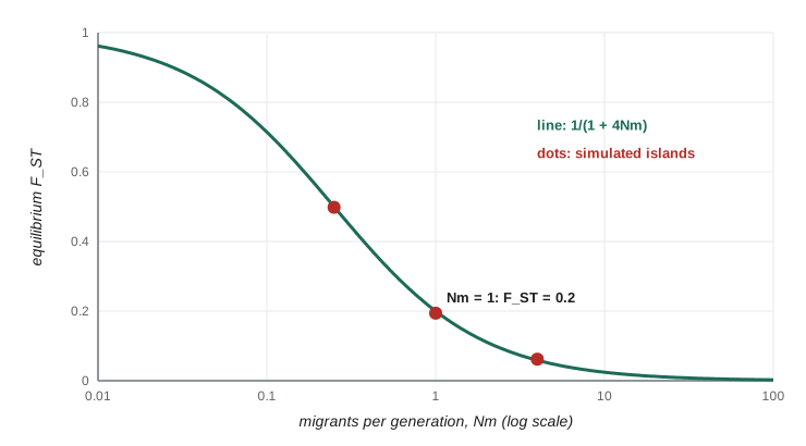
Wright’s island model imagines many subpopulations, each of N diploid individuals, exchanging migrants with a common pool at rate m per generation. Drift pushes subpopulations apart; migration pulls them together. At equilibrium, for neutral loci with low mutation rates:
The striking result is that equilibrium differentiation depends only on Nm, the number of migrants per generation, not on N or m separately. One migrant per generation (Nm = 1) gives F_ST = 0.2; ten give about 0.024. The rule of thumb that ‘one migrant per generation’ is enough to prevent strong divergence through drift, widely used in conservation management, comes from this formula. Recent work suggests that one to ten effective migrants per generation is a more realistic target for real populations, which depart from the model’s assumptions of equal sizes, symmetric migration and many islands.
import numpy as np
rng = np.random.default_rng(3227)

def island_fst(N, m, demes=20, loci=200, gens=1500):
    p = np.full((demes, loci), 0.5)
    for _ in range(gens):
        pbar = p.mean(axis=0)
        p = (1 - m) * p + m * pbar                     # migration from the common pool
        p = rng.binomial(2 * N, p) / (2 * N)           # drift within each island
    pbar = p.mean(axis=0)
    keep = (pbar > 0) & (pbar < 1)
    return np.sum(p[:, keep].var(axis=0)) / np.sum(pbar[keep] * (1 - pbar[keep]))

N = 50
for Nm in (0.25, 1, 4):
    print(f"Nm = {Nm:4}: simulated F_ST = {island_fst(N, Nm / N):.3f}, "
f"theory 1/(1 + 4Nm) = {1 / (1 + 4 * Nm):.3f}")Nm = 0.25: simulated F_ST = 0.498, theory 1/(1 + 4Nm) = 0.500 Nm = 1: simulated F_ST = 0.194, theory 1/(1 + 4Nm) = 0.200 Nm = 4: simulated F_ST = 0.062, theory 1/(1 + 4Nm) = 0.059
The simulations follow the approximation closely. Inverting the formula, Nm ≈ (1/F_ST − 1)/4, has been used countless times to estimate gene flow from F_ST, but Michael Whitlock and David McCauley warned in 1999 that real populations rarely meet the model’s assumptions, so such estimates should be treated as rough indices of connectivity, not literal counts of migrants. Lesson 8 introduces spatially explicit models and direct methods for studying gene flow.
Structure in human populations
Human populations are genetically structured, but weakly. Richard Lewontin’s 1972 analysis of blood-group and protein loci found that about 85 per cent of genetic variation lies within populations and only a small fraction among the major continental groupings, and genome-wide data have confirmed similar proportions. At the same time, because differences in allele frequency are small but consistent across hundreds of thousands of loci, statistical methods can assign many individuals to their broad region of origin with high accuracy. A. W. F. Edwards pointed out in 2003 that these two facts do not contradict each other: single loci are weakly informative, while many loci combined are informative. Neither fact supports treating ‘races’ as discrete biological groups. Human variation is mostly clinal, changing gradually with geography, and it is shaped by a history of migration and mixture, as lesson 8 explains. Genetic ancestry describes the geographic origins of segments of a genome; it is not the same as social categories of race or ethnicity.
Common mistakes
MistakeInterpreting a heterozygote deficit in a pooled sample as inbreeding.
InsteadIt may be a Wahlund effect from sampling across subpopulations; check F_IS within each subpopulation.
MistakeAveraging per-locus F_ST ratios across SNPs.
InsteadUse a ratio of averages: sum numerators and denominators across loci before dividing.
MistakeComparing F_ST values from microsatellites with those from SNPs.
InsteadHighly polymorphic markers cap F_ST; compare like with like or use standardized measures for allelic distinctness.
MistakeReading F_ST as time since populations split.
InsteadF_ST reflects drift relative to migration; small isolated populations diverge quickly.
MistakeConverting F_ST into a precise number of migrants.
InsteadThe island model’s assumptions are rarely met; treat Nm from F_ST as a rough index.
Summary and key terms
- Pooling subpopulations with different allele frequencies creates a heterozygote deficit equal to 2Var(p): the Wahlund effect.
- F_IS, F_ST and F_IT partition departures from Hardy–Weinberg proportions; (1 − F_IT) = (1 − F_IS)(1 − F_ST).
- Weir and Cockerham’s and Hudson’s estimators correct for sampling; combine loci as a ratio of averages.
- F_ST is capped by within-population heterozygosity, so values from different marker types are not comparable.
- F_ST = (T_B − T_W)/T_B links differentiation to coalescence times; under the island model F_ST ≈ 1/(1 + 4Nm).
- Human populations are weakly structured; variation is mostly within populations and mostly clinal.
- population structure
- Non-random distribution of genetic variation caused by subdivision and limited dispersal.
- Wahlund effect
- A heterozygote deficit in a pooled sample of subpopulations with different allele frequencies.
- F_IS
- The inbreeding coefficient of individuals relative to their subpopulation.
- F_ST
- The proportion of genetic variance due to differences among subpopulations.
- F_IT
- The inbreeding coefficient of individuals relative to the total population.
- Hudson’s F_ST
- A pairwise estimator based on within- and between-population heterozygosities.
- Jost’s D
- A measure of allelic differentiation that is not limited by within-population heterozygosity.
- island model
- A model of many equal subpopulations exchanging migrants with a common pool.
- Nm
- The number of migrants per generation, which determines equilibrium F_ST in the island model.
- Balding–Nichols model
- A beta-distribution model of subpopulation allele frequencies with variance F_ST p(1 − p).
Practice problems
Work each problem on paper first, then reveal the answer to check.
Two equally sized populations have p = 0.1 and 0.5. What heterozygote deficit appears in a pooled sample?
Show answer
Var(p) = 0.04, so the deficit is 0.08.
H_I = 0.30, H_S = 0.33 and H_T = 0.40. Calculate F_IS, F_ST and F_IT.
Show answer
F_IS ≈ 0.091, F_ST = 0.175, F_IT = 0.25.
Verify the relationship among the three F-statistics in the last answer.
Show answer
(1 − 0.091)(1 − 0.175) ≈ 0.75 = 1 − 0.25.
What is the largest possible F_ST when H_S = 0.8?
Show answer
0.2, since F_ST = 1 − H_S/H_T and H_T cannot exceed 1.
What equilibrium F_ST does the island model predict for Nm = 2?
Show answer
1/9 ≈ 0.11.
If F_ST = 0.05, what Nm does the island model imply?
Show answer
(20 − 1)/4 = 4.75 migrants per generation.
T_W = 1.0 and T_B = 1.25 units. What is F_ST?
Show answer
0.25/1.25 = 0.2.
Why can two recently separated populations have high F_ST?
Show answer
If they are small, drift changes their frequencies quickly.
Why should F_ST be averaged across loci as a ratio of averages?
Show answer
Averaging ratios gives too much weight to low-diversity loci and is biased.
How can most human genetic variation be within populations, yet individuals be assigned to regions accurately?
Show answer
Small frequency differences add up across many loci, so multilocus genotypes are informative even when each locus is not.
Lesson quiz · 5 questions
Score 60% or more to complete this lesson.
Create a free account to save your progress, take quizzes and earn a certificate.