
BIOL-322 · Lesson 12 of 12 · 31 min
Capstone: population genetics in conservation, forensics and human health
This final lesson brings the course together by applying its tools to three fields where population genetics shapes real decisions. In conservation, effective size, inbreeding and gene flow determine whether small populations can persist and whether moving animals between them will help. In forensic science, Hardy–Weinberg proportions, population structure and the product rule underlie the match probabilities presented in court. In human health, founder effects, linkage disequilibrium and polygenic prediction determine who is at risk of genetic disease and who benefits from genomic medicine, and questions of consent and governance determine whose genomes are studied at all. The lesson ends with a worked analysis of an invented dataset that draws on methods from every earlier lesson.
Genetic rescue
Small, isolated populations lose genetic variation through drift, become inbred and accumulate harmful mutations, as lessons 4 and 5 showed. Inbreeding depression can reduce survival and reproduction enough to push a population toward extinction, a feedback called the extinction vortex. Genetic rescue is the deliberate introduction of individuals from another population to restore variation and fitness. Its best-known example is the Florida panther, an isolated population of puma in southern Florida. By the early 1990s, fewer than about 30 adults remained, and they showed signs of inbreeding depression: kinked tails, undescended testes, heart defects and poor sperm quality. In 1995, eight female pumas from Texas, from the nearest population of the same species, were released into the Florida population. Five produced offspring. Over the following decade, heterozygosity roughly doubled, the signs of inbreeding became much less common in hybrid descendants, and survival improved; Florida’s wildlife agency has since estimated the adult population at roughly 120 to 230. Genetic studies have since warned that, without further gene flow, inbreeding will build up again, a reminder that rescue in a population that remains isolated must be repeated.
Genetic rescue has worked in many cases, including adders in Sweden, greater prairie chickens in Illinois and mountain pygmy possums in Australia, but managers long feared outbreeding depression, the loss of fitness when divergent populations interbreed. A decision framework published by Richard Frankham and colleagues in 2011 suggests that the risk is low when the populations belong to the same species, have the same chromosome arrangement, have been isolated for less than about 500 years and live in similar environments. Under those conditions, the expected benefit of restoring gene flow usually far outweighs the risk.
| Case (approximate figures) | Problem | Genetic intervention | Outcome |
|---|---|---|---|
| Florida panther (US) | Fewer than about 30 adults by early 1990s; inbreeding depression | Eight female Texas pumas released in 1995 | Heterozygosity and survival improved; numbers rose; further gene flow likely needed |
| Vancouver Island marmot (Canada) | Fewer than 30 in the wild in 2003 | Captive breeding from 1997 with pedigree management; releases to restore colonies | 427 wild marmots in 33 colonies counted by November 2025; about 120 in captivity |
| Wood bison (Canada) | Hunted to a few hundred animals by 1900; hybridization risk with plains bison | Disease-free, genetically screened herds such as Elk Island National Park used as sources for reintroductions | Many free-ranging herds re-established, including in Alaska in 2015 |
| Isle Royale wolves (US) | Severe inbreeding; population fell to two | Translocations of wolves from Canada and Minnesota from 2018 | Population re-established; genetic monitoring continues |
The Vancouver Island marmot, found only in the mountains of Vancouver Island, shows the role of captive breeding. In 2003, fewer than 30 animals remained in the wild. A captive breeding programme, begun in 1997 and run with zoos and a dedicated breeding centre, managed pairings by pedigree to keep the founders’ genetic contributions as even as possible, the principle of equalizing family sizes from lesson 4. By November 2025, the Marmot Recovery Foundation counted 427 marmots in the wild in 33 colonies, with about 120 more in captive breeding. Pedigree managers use mean kinship, the average coancestry of each animal with all others in the population, choosing animals with the lowest mean kinship as breeders, because they carry the rarest founder alleles.
Wood bison illustrate the importance of genetic distinctness. Hunting reduced them to a few hundred animals by about 1900, and later the transfer of plains bison into Wood Buffalo National Park in the 1920s created a risk of hybridization. A small, isolated group of wood bison discovered in the 1950s became the source of disease-free herds, including the herd at Elk Island National Park in Alberta, which has supplied animals for reintroductions across northern Canada and to Alaska and Russia. Genetic monitoring of these herds tracks heterozygosity and the effects of founding each new herd from a small number of animals.
import numpy as np
rng = np.random.default_rng(322)

def project(N, gens, migrants_every=0, k=0, L=500, reps=40):
    # expected heterozygosity of an isolated population with optional translocations
    out = np.zeros(gens + 1)
    for _ in range(reps):
        p = rng.uniform(0.2, 0.8, L)
        Hs = [np.mean(2 * p * (1 - p))]
        for g in range(1, gens + 1):
            p = rng.binomial(2 * N, p) / (2 * N)
            if migrants_every and g % migrants_every == 0:
                donor = rng.uniform(0.2, 0.8, L)          # frequencies in a large source population
                p = (1 - k / N) * p + (k / N) * donor
            Hs.append(np.mean(2 * p * (1 - p)))
        out += np.array(Hs)
    return out / reps

N, gens = 25, 40
iso = project(N, gens)
resc = project(N, gens, migrants_every=5, k=2)
for g in (0, 10, 20, 40):
    print(f"generation {g:2d}: H isolated = {iso[g]:.3f}, H with 2 migrants every 5 generations = {resc[g]:.3f}")
print(f"theory for the isolated population after 40 generations: {iso[0] * (1 - 1 / (2 * N)) ** 40:.3f}")generation 0: H isolated = 0.440, H with 2 migrants every 5 generations = 0.440 generation 10: H isolated = 0.359, H with 2 migrants every 5 generations = 0.392 generation 20: H isolated = 0.294, H with 2 migrants every 5 generations = 0.363 generation 40: H isolated = 0.198, H with 2 migrants every 5 generations = 0.339 theory for the isolated population after 40 generations: 0.196
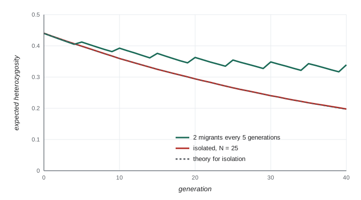
The projection shows why the ‘one migrant per generation’ rule from lesson 7 is a useful starting point: a few migrants every few generations stop the slide in heterozygosity. It also shows the scale of loss in an isolated population of 25, more than half of its heterozygosity in 40 generations, which for a mammal with a generation time of five years is only two centuries.
Forensic DNA profiles and match probabilities
A forensic DNA profile records the alleles at a set of highly polymorphic short tandem repeat loci. If a suspect’s profile matches the profile from a crime-scene sample, the court needs to know how surprising that match would be if the suspect were not the source. The random match probability is the probability that a randomly chosen unrelated person would have the same profile. Under Hardy–Weinberg proportions, the genotype frequency at each locus is p² for a homozygote and 2pq for a heterozygote, and if the loci are in linkage equilibrium, the probabilities multiply across loci, the product rule.
Population structure complicates the calculation, as lesson 7 explained. If the suspect and the true source belong to the same subpopulation, they are more likely to share alleles than two people drawn from the whole population. The US National Research Council’s 1996 report recommended a correction based on the Balding–Nichols model, using a value of θ (equivalent to F_ST) of 0.01 for most populations and up to 0.03 for small, isolated ones. With θ, the conditional match probability for a heterozygote A_iA_j becomes:
and for a homozygote A_iA_i, [2θ + (1 − θ)p_i][3θ + (1 − θ)p_i]/[(1 + θ)(1 + 2θ)]. The correction always makes the match probability larger, so it favours the defendant. The product rule with θ correction is standard in North American forensic laboratories.
import numpy as np

# an invented 10-locus STR profile with invented allele frequencies (not from any real database)
profile = [  # (frequency of allele 1, frequency of allele 2); equal values mean a homozygote
    (0.12, 0.21), (0.08, 0.08), (0.15, 0.30), (0.05, 0.11), (0.22, 0.22),
    (0.10, 0.17), (0.09, 0.26), (0.14, 0.14), (0.07, 0.19), (0.18, 0.25)]

def locus_prob(pi, pj, theta, homozygote):
    if homozygote:
        return (2*theta + (1 - theta)*pi) * (3*theta + (1 - theta)*pi) / ((1 + theta) * (1 + 2*theta))
    return 2 * (theta + (1 - theta)*pi) * (theta + (1 - theta)*pj) / ((1 + theta) * (1 + 2*theta))

for theta in (0.0, 0.01, 0.03):
    rmp = np.prod([locus_prob(a, b, theta, a == b) for a, b in profile])
print(f"theta = {theta:.2f}: random match probability = {rmp:.2e} (about 1 in {1 / rmp:,.0f})")theta = 0.00: random match probability = 1.15e-15 (about 1 in 866,570,590,173,757) theta = 0.01: random match probability = 6.15e-15 (about 1 in 162,701,029,205,241) theta = 0.03: random match probability = 8.92e-14 (about 1 in 11,215,278,848,750)
Even with the most conservative θ, the random match probability for ten loci is tiny. Modern kits type 20 or more loci, which can push the probability for unrelated people below one in a trillion trillion. Two cautions keep these numbers in perspective. First, the probability of a match between relatives is far higher: full siblings share both alleles at a locus with probability about 1/4, so a match probability calculation must consider whether a relative could be the source. Second, the match probability is not the probability that the defendant is innocent. Confusing the two is the prosecutor’s fallacy; the chance that the sample came from someone else also depends on laboratory error, contamination, and the number of plausible alternative sources.
In Canada, the National DNA Data Bank (NDDB), operated by the RCMP under the DNA Identification Act, began operating in 2000. It holds a Convicted Offenders Index of profiles from people convicted of designated offences and a Crime Scene Index of profiles from unsolved cases, and since 2018 it has also held humanitarian indices for missing persons, human remains and voluntary donations from relatives of missing persons. The RCMP’s statistics page, consulted in October 2026, reported about 507,600 profiles in the Convicted Offenders Index, about 269,500 in the Crime Scene Index and more than 110,000 matches since the bank opened. The equivalent US system, CODIS, run by the FBI, has used 20 core STR loci since 2017 and holds many millions of profiles. Canadian law strictly limits how NDDB profiles may be used, and searching for partial matches to relatives for criminal investigations is far more restricted than in some US states.
Investigative genetic genealogy, which compares crime-scene DNA with profiles that people have uploaded to consumer genealogy databases and then builds family trees to identify candidates, became prominent after the 2018 arrest in the Golden State Killer case. It uses hundreds of thousands of SNPs and the lengths of shared chromosome segments, the identity-by-descent logic of lesson 8, to estimate relationships as distant as third cousins. It raises new questions about consent, because the people whose profiles lead investigators to a suspect are usually relatives who never agreed to take part.
Founder effects and human health
Population history shapes the distribution of disease alleles. When a population descends from a small number of founders and then grows rapidly, alleles carried by a founder can reach unusually high frequencies, as lesson 4 explained. In Quebec, settlement by roughly 8,500 French immigrants in the seventeenth and eighteenth centuries, followed by rapid growth and regional founder events, raised the frequencies of several recessive disorders. Hereditary tyrosinemia type 1, for example, is far more common in the Saguenay–Lac-Saint-Jean region than elsewhere, and newborn screening and carrier testing programmes were designed around this regional pattern. Similar founder effects are seen among Ashkenazi Jewish, Finnish, Amish and Hutterite populations. Knowing the population history makes targeted screening far more efficient, because a few founder variants can account for most cases.
Worked problem
Carrier frequency from disease incidence
A recessive disorder affects about 1 in 2,000 births in a region. Assuming Hardy–Weinberg proportions, what fraction of people are carriers, and what is the chance that two random people from the region are both carriers?
Show solution
- q² = 1/2,000 = 0.0005, so q ≈ 0.0224.
- Carrier frequency 2pq ≈ 2 × 0.978 × 0.0224 ≈ 0.044, or about 1 in 23.
- Probability both partners are carriers ≈ 0.044² ≈ 0.0019, about 1 in 520.
- Each child of two carriers has a 1/4 chance of being affected, which returns the incidence of 1 in about 2,000.
Answer: About 1 in 23 people are carriers, and about 1 couple in 520 is at risk; targeted carrier screening can identify these couples before they have children.
Diversity, governance and Indigenous genomics
Lesson 11 showed that genomic tools work best for people whose ancestry is well represented in research. Indigenous peoples have been particularly underrepresented, partly because of a history of research conducted without meaningful consent or benefit. Correcting this requires more than recruiting participants; it requires that communities govern how their samples and data are used.
Silent Genomes, a project funded by Genome Canada and Genome British Columbia, is one response. Led in partnership with First Nations, Inuit and Métis peoples, it aims to reduce inequities in the genetic diagnosis of Indigenous children with genetic diseases by building an Indigenous Background Variant Library, a reference of genetic variation that lets clinicians recognize which variants are common and likely harmless in Indigenous populations, under Indigenous governance of samples and data. Without such a reference, variants that are common in a community but absent from European-dominated databases can be mistaken for causes of disease, which delays correct diagnosis.
In Canada, research involving First Nations, Inuit and Métis communities is governed by Chapter 9 of the Tri-Council Policy Statement (TCPS 2), which requires community engagement, and many First Nations apply the OCAP® principles of ownership, control, access and possession over their data. The CARE principles for Indigenous data governance, published by the Global Indigenous Data Alliance in 2019, complement the FAIR principles for data sharing by adding Collective benefit, Authority to control, Responsibility and Ethics.
Capstone analysis: an invented dataset
The final analysis applies tools from across the course to an invented dataset. Two populations of an invented endangered amphibian, the ‘Corrie Lake newt’, live in ponds 40 kilometres apart. Population A (60 breeding adults counted) is isolated; population B (400 adults) is larger. Both were genotyped at 300 SNPs in 2016 and 2024, with about four generations in between. The questions are typical of a real conservation genetic assessment: how much diversity does each population have, are they inbred, how differentiated are they, what is the effective size of the small population, and would moving animals from B to A help?
import numpy as np
rng = np.random.default_rng(3222)

L, gens = 300, 4
anc = rng.uniform(0.1, 0.9, L)
def bn(p, F):
    return rng.beta(p * (1 - F) / F, (1 - p) * (1 - F) / F)
pA0, pB0 = bn(anc, 0.10), bn(anc, 0.02)            # invented histories: A more drifted
NeA, NeB = 18, 150                                  # invented true effective sizes
pA1, pB1 = pA0.copy(), pB0.copy()
for _ in range(gens):
    pA1 = rng.binomial(2 * NeA, pA1) / (2 * NeA); pB1 = rng.binomial(2 * NeB, pB1) / (2 * NeB)

def sample(p, n, F=0.0):
    # genotypes (0, 1 or 2 copies) with inbreeding coefficient F
    q = 1 - p
    P0 = q * q + F * p * q; P1 = 2 * p * q * (1 - F)
    u = rng.random((n, len(p)))
    return np.where(u < P0, 0, np.where(u < P0 + P1, 1, 2))
nA = nB = 40
GA0, GA1 = sample(pA0, nA, 0.06), sample(pA1, nA, 0.06)
GB1 = sample(pB1, nB)

def stats(G):
    n = len(G); p = G.sum(0) / (2 * n)
    Ho = np.mean(G == 1); He = np.mean(2 * n / (2 * n - 1) * 2 * p * (1 - p))
    return p, Ho, He, 1 - Ho / He
pa0, *_ = stats(GA0)
pa1, HoA, HeA, FA = stats(GA1)
pb1, HoB, HeB, FB = stats(GB1)
print(f"2024 population A: Ho = {HoA:.3f}, He = {HeA:.3f}, F = {FA:.3f}")
print(f"2024 population B: Ho = {HoB:.3f}, He = {HeB:.3f}, F = {FB:.3f}")

hw = pa1 * (1 - pa1) + pb1 * (1 - pb1); hb = pa1 * (1 - pb1) + pb1 * (1 - pa1)
print(f"Hudson F_ST between A and B (2024) = {1 - hw.sum() / hb.sum():.3f}")

z = (pa0 + pa1) / 2; keep = (z > 0.05) & (z < 0.95)
Fc = np.mean((pa0[keep] - pa1[keep]) ** 2 / (z[keep] * (1 - z[keep])))
Ne_hat = gens / (2 * (Fc - 1 / (2 * nA) - 1 / (2 * nA)))
print(f"temporal estimate of Ne for A = {Ne_hat:.0f} (census 60; invented true value {NeA})")2024 population A: Ho = 0.304, He = 0.328, F = 0.073 2024 population B: Ho = 0.387, He = 0.383, F = -0.009 Hudson F_ST between A and B (2024) = 0.127 temporal estimate of Ne for A = 18 (census 60; invented true value 18)
The analysis tells a coherent story. Population A has lower heterozygosity than B and a positive F, consistent with mating among relatives in a small population. The two populations are moderately differentiated. The temporal estimate of A’s effective size is far below its census size of 60, in line with the typical N_e/N ratios of lesson 4, though with only 40 individuals sampled at each time and four generations the confidence interval would be wide. With an effective size this small, A would lose about 3 per cent of its heterozygosity per generation. The populations belong to the same species, live in similar habitat and were presumably connected until recently, so Frankham’s decision framework suggests a low risk of outbreeding depression. The recommended management would be to translocate a few adults from B to A every generation or two, to restore pond connectivity if possible, and to repeat genetic monitoring to measure the response. Because these data are invented, the specific numbers illustrate the workflow only; a real assessment would also report confidence intervals, check for null alleles and related individuals, and consider demographic and ecological evidence.
Common mistakes
MistakeAssuming one genetic rescue solves the problem permanently.
InsteadIf isolation continues, drift and inbreeding resume; plan for repeated gene flow and monitoring.
MistakeRefusing translocations out of fear of outbreeding depression in every case.
InsteadThe risk is low for recently isolated populations of the same species in similar environments.
MistakeCalculating a match probability without accounting for population structure or relatives.
InsteadApply the θ correction and consider whether a relative could be the source.
MistakeEquating the random match probability with the probability of innocence.
InsteadThat is the prosecutor’s fallacy; other evidence and alternative sources matter.
MistakeTreating representation in genomic research as only a recruitment problem.
InsteadCommunity governance of samples and data, as in the CARE principles and Silent Genomes, is essential.
Summary and key terms
- Genetic rescue restores variation and fitness to inbred populations, as in the Florida panther, but must be repeated if isolation continues.
- Pedigree management by mean kinship and equalized family sizes conserves founder diversity in captive programmes such as the Vancouver Island marmot’s.
- Random match probabilities use the product rule with a θ correction for population structure; relatives and the prosecutor’s fallacy require care.
- National DNA databases differ in loci, scope and rules on familial searching.
- Founder effects raise the frequency of particular disease alleles and allow targeted screening.
- Indigenous-led governance, as in Silent Genomes and the CARE principles, is central to equitable genomics.
- genetic rescue
- Introducing individuals into a small, inbred population to restore genetic variation and fitness.
- extinction vortex
- A feedback in which small size, inbreeding and demographic chance drive a population toward extinction.
- outbreeding depression
- Reduced fitness in offspring of crosses between divergent populations.
- mean kinship
- The average coancestry of an individual with all members of a managed population.
- random match probability
- The probability that a randomly chosen unrelated person has a given DNA profile.
- product rule
- Multiplying genotype frequencies across loci to obtain a profile frequency.
- prosecutor’s fallacy
- Confusing the probability of a match given innocence with the probability of innocence given a match.
- familial searching
- Searching a DNA database for partial matches that may indicate a relative of the source of a sample.
- founder effect
- Changes in allele frequencies when a population descends from a small number of founders.
- CARE principles
- Principles for Indigenous data governance: Collective benefit, Authority to control, Responsibility and Ethics.
Practice problems
Work each problem on paper first, then reveal the answer to check.
An isolated population of N_e = 20 starts with H = 0.4. What H is expected after 20 generations?
Show answer
0.4 × (1 − 1/40)^20 ≈ 0.4 × 0.60 ≈ 0.24.
Why should breeders with the lowest mean kinship be chosen?
Show answer
They carry the rarest founder alleles, so breeding them conserves diversity.
A heterozygote has alleles with frequencies 0.1 and 0.2. What is its genotype frequency with θ = 0?
Show answer
2 × 0.1 × 0.2 = 0.04.
What is the homozygote probability for an allele with p = 0.1 and θ = 0.01?
Show answer
[0.02 + 0.099][0.03 + 0.099]/(1.01 × 1.02) ≈ 0.119 × 0.129/1.0302 ≈ 0.0149.
Does the θ correction make match probabilities larger or smaller?
Show answer
Larger, which is conservative toward the defendant.
What is the prosecutor’s fallacy?
Show answer
Treating the probability of a match if the suspect is innocent as the probability that the suspect is innocent.
A recessive disease affects 1 in 10,000 births. What is the carrier frequency?
Show answer
q = 0.01; 2pq ≈ 0.0198, about 1 in 50.
Why are founder populations useful for targeted genetic screening?
Show answer
A few founder variants account for most cases, so testing for them is efficient.
What is the purpose of an Indigenous Background Variant Library?
Show answer
To let clinicians recognize common, likely harmless variants in Indigenous populations and so diagnose genetic disease more accurately.
Name the four CARE principles.
Show answer
Collective benefit, Authority to control, Responsibility and Ethics.
Lesson quiz · 5 questions
Score 60% or more to complete this lesson.
Create a free account to save your progress, take quizzes and earn a certificate.