
BIOL-322 · Lesson 6 of 12 · 26 min
The coalescent and neutral diversity statistics
Classical population genetics looks forward in time: given allele frequencies now, what will they be in the next generation? With DNA sequence data, it is often more natural to look backward. A sample of sequences has a genealogy, a tree describing how their lineages merge into common ancestors as we trace them into the past. Coalescent theory, introduced by John Kingman in 1982 and developed by Richard Hudson, Fumio Tajima and others, describes the shape of that genealogy under neutral evolution. It is the mathematical foundation of modern population genomics: it explains why the site frequency spectrum of lesson 1 is proportional to 1/i, provides two estimators of the population mutation rate, and gives a test of neutrality, Tajima’s D, that compares them. It also makes simulation of genomic data fast enough to fit complex demographic models.
Two lineages
Take two gene copies sampled from a Wright–Fisher population of 2N copies. In the previous generation, each copy had a parent chosen at random from the 2N copies, so the chance that both came from the same parent, that their lineages coalesce, is 1/(2N). If they do not coalesce, the same reasoning applies one generation further back. The number of generations until coalescence therefore follows a geometric distribution with mean 2N. When N is large it is well approximated by an exponential distribution with mean 2N generations. It is conventional to measure coalescent time in units of 2N generations (or 2N_e when the population is not ideal), so that the expected time for two lineages to coalesce is 1.
This simple result already explains the relationship between diversity and the mutation rate. Two sequences differ at every site where a mutation occurred on either branch since their common ancestor. The total branch length connecting them is twice the coalescence time, on average 4N generations, so with μ neutral mutations per site per generation, the expected number of differences per site is 4Nμ = θ. Nucleotide diversity, π, is therefore an estimator of θ, as lesson 5 assumed.
Many lineages
With k lineages, any of the k(k − 1)/2 pairs could coalesce. In coalescent time units, each pair coalesces at rate 1, so the waiting time until the first coalescence among k lineages is exponential with rate k(k − 1)/2 and mean 2/[k(k − 1)]. After that event, k − 1 lineages remain, and the process repeats until a single lineage, the most recent common ancestor (MRCA) of the sample, is reached. Two features follow immediately. The last stage, when only two lineages remain, is the longest, with expected duration 1. And adding more sequences to a sample mostly adds short branches near the tips:
in units of 2N generations. The expected time to the MRCA of a sample of 10 is already 1.8 units, 90 per cent of the value for an infinitely large sample. Sampling more individuals barely changes how far back the genealogy reaches. This is why even a small sample of genomes contains information about the deep history of a population, and why large samples are mainly useful for studying rare, recent variation.
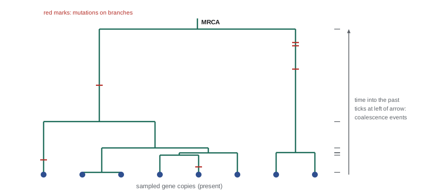
Mutations on the genealogy and the site frequency spectrum
Under neutrality, mutations do not affect the genealogy; they simply fall on its branches at a constant rate, like raindrops on a tree. A mutation on a branch is inherited by every sampled sequence below that branch. Under the infinite-sites model, each mutation produces one segregating site, and its derived allele count is the number of descendants of the branch it fell on. This view makes the site frequency spectrum easy to understand. Mutations on the external branches leading to single tips produce singletons; mutations on branches subtending two tips produce doubletons; and so on. Fu showed in 1995 that the expected total length of branches with i descendants is proportional to 1/i, which is the 1/i spectrum of lesson 1.
Demographic history changes the shape of the genealogy and therefore the spectrum. In a population that has grown rapidly, coalescence rates were low in the recent past, when the population was large, and high further back, when it was small. The genealogy is star-like, with long external branches and short internal ones, producing an excess of singletons. A bottleneck or a population subdivided into isolated groups does the opposite: lineages coalesce quickly within groups or during the bottleneck, but the last few lineages take a long time to merge, giving long internal branches and an excess of intermediate-frequency variants.
Two estimators of θ
The coalescent gives two estimators of θ that use different aspects of the data. The first is π itself: the average number of pairwise differences, which has expectation θ (per site or per locus). The second, proposed by G. A. Watterson in 1975, uses the number of segregating sites S. Because the expected total branch length is 2Σ1/i in units of 2N generations, and mutations accumulate at rate θ/2 per unit of branch length, the expected number of segregating sites is θ times a_n = Σ1/i, summed from i = 1 to n − 1:
Both estimators have expectation θ under the standard neutral model with constant size, but they weight variants differently. Watterson’s estimator counts every segregating site equally, so it is sensitive to rare variants, which make up most segregating sites. π weights each site by the number of pairwise differences it creates, c(n − c) for a derived allele in c of n sequences, so intermediate-frequency variants contribute most.
Worked problem
Computing θ_W and π
Ten sequences (n = 10) of a 1,000-base region contain S = 14 segregating sites. The derived allele counts at these sites are: six singletons, three doubletons, two sites at 3, one at 5, one at 7 and one at 9. Calculate θ_W and π per site.
Show solution
- a_10 = 1 + 1/2 + … + 1/9 ≈ 2.829, so θ_W = 14/2.829 ≈ 4.95 per region, or 0.00495 per site.
- Pairwise differences per site with derived count c: c(10 − c). Singletons give 9 each, doubletons 16, count 3 gives 21, count 5 gives 25, count 7 gives 21 and count 9 gives 9.
- Total = 6 × 9 + 3 × 16 + 2 × 21 + 25 + 21 + 9 = 54 + 48 + 42 + 55 = 199.
- Number of pairs = 45, so π = 199/45 ≈ 4.42 per region, or 0.00442 per site.
- π is below θ_W, so the sample has somewhat more rare variants than expected.
Answer: θ_W ≈ 0.0050 and π ≈ 0.0044 per site; the difference is modest and may not be significant, which Tajima’s D can assess.
Tajima’s D
In 1989 Fumio Tajima proposed comparing the two estimators. His statistic D is the difference π − θ_W divided by an estimate of its standard deviation under the neutral model:
Here e_1 and e_2 are constants that depend only on the sample size. Under the standard neutral model, D has a mean near zero and lies roughly between −2 and 2 most of the time. Negative D means an excess of rare variants, as produced by population growth, by a recent selective sweep (which wipes out variation and leaves new, rare mutations accumulating afterwards) or by purifying selection removing deleterious variants before they reach intermediate frequency. Positive D means an excess of intermediate-frequency variants, as produced by balancing selection, by a population bottleneck or by population structure.
| Pattern | Tajima’s D | Possible demographic explanation | Possible selective explanation |
|---|---|---|---|
| Excess of rare variants | Negative | Recent population growth | Recent selective sweep; purifying selection |
| Close to neutral expectation | Near zero | Constant size, random mating | Neutral evolution |
| Excess of intermediate variants | Positive | Bottleneck; population structure; sampling from several groups | Balancing selection |
The table shows the central difficulty in using D. Demography and selection can produce the same signal. The way out is to compare loci: demographic history affects the whole genome, while selection affects particular regions. A genome-wide average D of −0.5 in a population that has expanded, with a handful of genes showing D below −2, is more informative than any single value. Human populations outside Africa generally show more negative genome-wide D than many African populations because of the combined effects of the out-of-Africa bottleneck and subsequent rapid growth.
import numpy as np
rng = np.random.default_rng(322)

def tajima_D(counts, n):
    counts = np.asarray(counts); S = len(counts)
    i = np.arange(1, n)
    a1, a2 = np.sum(1/i), np.sum(1/i**2)
    b1 = (n + 1) / (3*(n - 1)); b2 = 2*(n*n + n + 3) / (9*n*(n - 1))
    c1 = b1 - 1/a1; c2 = b2 - (n + 2)/(a1*n) + a2/a1**2
    e1 = c1/a1; e2 = c2/(a1**2 + a2)
    pi = np.sum(counts*(n - counts)) / (n*(n - 1)/2)
    return pi, S/a1, (pi - S/a1) / np.sqrt(e1*S + e2*S*(S - 1))

def coalescent(n, theta):
    # returns derived-allele counts for each mutation on one neutral genealogy
    lineages = [frozenset([k]) for k in range(n)]
    counts = []
    while len(lineages) > 1:
        k = len(lineages)
        t = rng.exponential(2 / (k*(k - 1)))      # time in units of 2N generations
        for lin in lineages:                       # mutations at rate theta/2 per branch
            counts += [len(lin)] * rng.poisson(theta/2 * t)
        a, b = sorted(rng.choice(k, 2, replace=False), reverse=True)
        merged = lineages.pop(a) | lineages.pop(b)
        lineages.append(merged)
    return counts

n, theta = 10, 5.0
print("worked example:  pi = %.2f, theta_W = %.2f, D = %.2f" %
      tajima_D([1]*6 + [2]*3 + [3]*2 + [5, 7, 9], n))

D_vals, S_vals, pi_vals = [], [], []
for _ in range(4000):
    c = coalescent(n, theta)
    if len(c) > 1:
        p, w, d = tajima_D(c, n); D_vals.append(d); S_vals.append(len(c)); pi_vals.append(p)
print(f"neutral simulations: mean S = {np.mean(S_vals):.2f} (expected {theta*np.sum(1/np.arange(1,n)):.2f}), "
      f"mean pi = {np.mean(pi_vals):.2f} (expected {theta:.2f})")
print(f"mean D = {np.mean(D_vals):.2f}; 2.5% and 97.5% quantiles = {np.percentile(D_vals, 2.5):.2f}, {np.percentile(D_vals, 97.5):.2f}")worked example: pi = 4.42, theta_W = 4.95, D = -0.49 neutral simulations: mean S = 14.31 (expected 14.14), mean pi = 5.06 (expected 5.00) mean D = -0.06; 2.5% and 97.5% quantiles = -1.74, 1.70
The worked example gives a D well inside the range of neutral simulations, so the slight excess of rare variants is not significant. The simulations also confirm the coalescent expectations for S and π. Simulating a null distribution like this, ideally under a demographic model fitted to genome-wide data, is how modern analyses judge whether a particular locus is unusual. Specialized software such as msprime simulates whole chromosomes with recombination for thousands of genomes in seconds, using the same principles as this short function.
Recombination and the ancestral recombination graph
So far each locus has had a single genealogy. Recombination means that different segments of a chromosome can have different genealogies, because, going back in time, a recombination event splits a lineage into two parents. The full history of a recombining chromosome is called the ancestral recombination graph. Nearby sites share almost the same tree; distant sites have nearly independent trees. This has two practical consequences. First, each independent stretch of the genome provides a new sample of the coalescent process, so a single diploid genome contains information about many genealogies. Second, because coalescence times vary along the genome, the density of heterozygous sites in one genome can be used to reconstruct how N_e changed over time.
The pairwise sequentially Markovian coalescent (PSMC) method of Heng Li and Richard Durbin, published in 2011, does exactly this. In regions where the two copies of a chromosome in one person coalesced long ago, heterozygous sites are dense; where they coalesced recently, sites are sparse. Converting the distribution of coalescence times into a history of N_e shows, for example, a reduction in the effective size of non-African human populations roughly 50,000 to 100,000 years ago, consistent with the out-of-Africa bottleneck. PSMC has been applied to hundreds of species, from mammoths to birds, and newer methods use many genomes at once to resolve more recent history. Converting coalescent time units into years requires assumed values for the mutation rate and generation time, so absolute dates carry considerable uncertainty.
Common mistakes
MistakeExpecting a much larger sample to reach much further back in time.
InsteadThe expected time to the MRCA of n sequences is 2(1 − 1/n), which is already 90 per cent of its maximum for n = 10.
MistakeTreating π and θ_W as different quantities.
InsteadBoth estimate θ under neutrality; their difference is what carries information about demography and selection.
MistakeConcluding that negative Tajima’s D proves positive selection.
InsteadPopulation growth and purifying selection also produce negative D; compare the locus with the genome-wide distribution.
MistakeConverting PSMC curves to years without stating assumptions.
InsteadDates depend on assumed mutation rates and generation times; report them and their uncertainty.
MistakeAssuming one genealogy describes a whole chromosome.
InsteadRecombination gives different segments different genealogies, described by the ancestral recombination graph.
Summary and key terms
- Two lineages coalesce after an exponential time with mean 2N_e generations; with k lineages the rate is k(k − 1)/2 per 2N_e generations.
- The expected time to the MRCA of n sequences is 2(1 − 1/n) units, so most of the genealogy’s depth comes from the last two lineages.
- Neutral mutations fall on branches like rain; branch lengths explain the 1/i site frequency spectrum.
- Watterson’s θ_W = S/a_n and nucleotide diversity π both estimate θ = 4N_eμ under neutrality.
- Tajima’s D compares π with θ_W; negative values indicate excess rare variants and positive values excess intermediate variants.
- Recombination gives each genomic segment its own genealogy, which PSMC and related methods use to infer histories of N_e.
- coalescent
- A model of the genealogy of a sample traced backward in time to its common ancestor.
- coalescence
- The merging of two lineages into their common ancestor.
- most recent common ancestor
- The single ancestral gene copy from which all sequences in a sample descend.
- segregating site
- A site that is polymorphic in the sample.
- Watterson’s estimator
- θ_W = S/a_n, an estimate of θ from the number of segregating sites.
- Tajima’s D
- A standardized difference between π and θ_W used to test the standard neutral model.
- star-like genealogy
- A genealogy with long external branches and short internal ones, typical of rapid growth.
- ancestral recombination graph
- The structure that records genealogies and recombination events along a chromosome.
- PSMC
- A method that infers past effective population sizes from the distribution of heterozygous sites in one genome.
- external branch
- A branch of a genealogy leading to a single sampled sequence.
Practice problems
Work each problem on paper first, then reveal the answer to check.
What is the expected coalescence time of two lineages in a population with N_e = 5,000?
Show answer
2N_e = 10,000 generations.
With 6 lineages, what is the expected waiting time to the first coalescence, in units of 2N_e generations?
Show answer
2/(6 × 5) = 1/15 ≈ 0.067.
What is the expected time to the MRCA of 20 sequences?
Show answer
2(1 − 1/20) = 1.9 units of 2N_e generations.
Calculate a_n for n = 5.
Show answer
1 + 1/2 + 1/3 + 1/4 ≈ 2.083.
A sample of 5 sequences has S = 10. What is θ_W?
Show answer
10/2.083 ≈ 4.8 per locus.
How many pairwise differences does a site with derived count 3 contribute in a sample of 8?
Show answer
3 × 5 = 15.
A locus has π = 3.1 and θ_W = 5.0. What sign will Tajima’s D have?
Show answer
Negative.
Give one demographic and one selective cause of positive Tajima’s D.
Show answer
A bottleneck or population structure; balancing selection.
Why does a rapidly growing population have an excess of singletons?
Show answer
Its genealogy is star-like, with long external branches that collect many mutations unique to one sequence.
What information does PSMC use?
Show answer
The varying density of heterozygous sites along one diploid genome, which reflects local coalescence times.
Lesson quiz · 5 questions
Score 60% or more to complete this lesson.
Create a free account to save your progress, take quizzes and earn a certificate.