
BIOL-214 · Lesson 1 of 12 · 33 min
Studying cells: modern microscopy and quantitative cell biology
Cell biology is the study of how cells are organized and how their parts work together. Earlier courses introduced the basic tour: BIOL-107 described the organelles of a typical eukaryotic cell, the light and electron microscopes, cell fractionation and the limits set by the wavelength of light. This course goes inside each compartment in depth, asking how a cell builds and maintains its internal organization, how proteins find their way to the right place, how the cytoskeleton shapes and moves the cell, how cells stick together and talk to each other, and how they decide when to divide or die. Throughout, the emphasis is quantitative: how big, how many, how fast. This first lesson is about the tools that make such questions answerable. Modern cell biology rests on fluorescent probes that label specific molecules in living cells, on microscopes that beat the classical limit of resolution, on cryo-electron methods that show molecular machines in their natural setting, and on image analysis that turns pictures into numbers.
Why measurement matters
For most of the twentieth century, cell biology was largely descriptive. Electron micrographs of the 1950s and 1960s, many made by George Palade, Keith Porter and their colleagues, revealed the endoplasmic reticulum, the Golgi apparatus, mitochondrial cristae and the double nuclear envelope. These images defined the compartments that this course is about. But a picture of a fixed cell is a single frame from a film, and it does not say how fast molecules move, how many copies of a protein are present or how long a structure lasts. Today the questions are dynamic and quantitative. How quickly does a membrane protein diffuse? What fraction of a receptor sits on the cell surface rather than inside? How many microtubules grow from a centrosome each minute? Answering them requires both the right probes and careful measurement.
A useful starting point is to know how large a typical cell is and how its volume and membranes are divided among compartments. Morphometric studies, which estimate volumes and areas from many thin sections using the principles of stereology, have given such numbers for well-studied cells such as rat liver hepatocytes and pancreatic acinar cells.
| Compartment | Share of cell volume (approx.) | Share of total membrane (approx.) |
|---|---|---|
| Cytosol | 54 % | None (no membrane) |
| Mitochondria | 22 % | 39 % (outer 7 %, inner 32 %) |
| Rough endoplasmic reticulum | 9 % | 35 % |
| Smooth ER and Golgi | 6 % | 23 % (smooth ER 16 %, Golgi 7 %) |
| Nucleus | 6 % | Under 1 % |
| Peroxisomes | 1 % | Under 1 % |
| Lysosomes | 1 % | Under 1 % |
| Endosomes | 1 % | Under 1 % |
| Plasma membrane | Not applicable | About 2 % |
Two lessons stand out from such data. First, internal membranes vastly outnumber the plasma membrane: in a hepatocyte, the plasma membrane is only about 2 per cent of the total membrane area, and the endoplasmic reticulum alone accounts for half. Second, membranes and organelles occupy nearly half of the cell, so the cytoplasm is not a bag of fluid but a densely packed, structured space.
# Stereology: converting volume and membrane fractions into absolute amounts
# Illustrative hepatocyte: volume about 5,000 um^3,
# total membrane area about 110,000 um^2 (approximate textbook values)
cell_volume = 5000.0      # um^3
total_membrane = 110000.0 # um^2

volume_fraction = {"cytosol": 0.54, "mitochondria": 0.22, "rough ER": 0.09,
                   "smooth ER + Golgi": 0.06, "nucleus": 0.06, "peroxisomes": 0.01,
                   "lysosomes": 0.01, "endosomes": 0.01}
membrane_fraction = {"plasma membrane": 0.02, "rough ER": 0.35, "smooth ER": 0.16,
                     "Golgi": 0.07, "mitochondrial outer": 0.07, "mitochondrial inner": 0.32}

for name, f in volume_fraction.items():
    print(f"{name:22s} {f*100:4.0f}%  ~{f*cell_volume:7.0f} um^3")
print()
for name, f in membrane_fraction.items():
    print(f"{name:22s} {f*100:4.0f}%  ~{f*total_membrane:8.0f} um^2")

# How many times larger is the ER membrane than the plasma membrane?
er = membrane_fraction["rough ER"] + membrane_fraction["smooth ER"]
print(f"\nER membrane / plasma membrane = {er / membrane_fraction['plasma membrane']:.0f}x")cytosol 54% ~ 2700 um^3 mitochondria 22% ~ 1100 um^3 rough ER 9% ~ 450 um^3 smooth ER + Golgi 6% ~ 300 um^3 nucleus 6% ~ 300 um^3 peroxisomes 1% ~ 50 um^3 lysosomes 1% ~ 50 um^3 endosomes 1% ~ 50 um^3 plasma membrane 2% ~ 2200 um^2 rough ER 35% ~ 38500 um^2 smooth ER 16% ~ 17600 um^2 Golgi 7% ~ 7700 um^2 mitochondrial outer 7% ~ 7700 um^2 mitochondrial inner 32% ~ 35200 um^2 ER membrane / plasma membrane = 26x
Fluorescent proteins changed everything
The single most important tool of modern cell biology is the ability to make a specific protein glow inside a living cell. In 1962 Osamu Shimomura purified green fluorescent protein (GFP) from the jellyfish Aequorea victoria. In 1994 Martin Chalfie showed that the cloned GFP gene could be expressed in other organisms, producing fluorescence without any added cofactor, and Roger Tsien engineered variants with brighter fluorescence and new colours. The three shared the 2008 Nobel Prize in Chemistry. Today a researcher can fuse the coding sequence of a fluorescent protein to the gene of interest, often at the gene’s natural location using genome editing (BIOL-207), and watch the tagged protein move through the living cell.
Fluorescence works because a fluorophore absorbs light of one wavelength and emits light of a longer wavelength a few nanoseconds later. Filters separate the dim emitted light from the much brighter excitation light, so labelled structures appear bright on a dark background. Several colours can be used together. Besides fluorescent proteins, cell biologists use antibodies carrying synthetic dyes (immunofluorescence), small dyes that bind particular structures, such as DAPI for DNA and phalloidin for actin filaments, and self-labelling protein tags such as HaloTag and SNAP-tag, which bind bright synthetic dyes added to the cells. Biosensors are engineered fluorescent proteins whose brightness or colour changes when they bind calcium, cyclic AMP or another signal, or when a kinase phosphorylates them, so that signalling events can be watched in real time.
A tag can change the behaviour of the protein it marks. A fluorescent protein is about 27 kDa, as large as many of the proteins it labels, and it can block a targeting signal at one end or interfere with binding partners. Careful experiments test whether the tagged protein still works, for example by showing that it rescues cells lacking the untagged version.
Beyond the widefield microscope
In a conventional widefield fluorescence microscope, light from out-of-focus planes blurs the image of thick specimens. Several designs reduce this blur.
| Method | How it works | Strengths | Typical use |
|---|---|---|---|
| Confocal (laser scanning or spinning disk) | A pinhole rejects light from out-of-focus planes | Sharp optical sections; 3D stacks | Fixed and living cells and tissues |
| Two-photon | Two infrared photons excite a fluorophore only at the focus | Deep tissue imaging with less damage | Living brain and organ slices |
| Light-sheet | A thin sheet of light illuminates only the plane being imaged | Fast, gentle imaging of whole embryos | Development over hours or days |
| TIRF | Light reflected at the coverslip excites only about 100 nm into the cell | Very low background at the cell surface | Vesicle fusion, receptor clustering |
| Super-resolution (STED, SIM, PALM/STORM) | Different tricks bypass the diffraction limit | Resolution of 20–120 nm | Nanoscale organization of molecules |
Breaking the diffraction limit
As BIOL-107 explained, a lens cannot focus light to a point smaller than about half its wavelength. For green light and a good oil-immersion objective, the lateral resolution is roughly 200 to 250 nm, which is larger than many of the structures cell biologists care about: a ribosome is about 25 nm across, a microtubule 25 nm and a synaptic vesicle 40 nm.
Super-resolution methods, recognized by the 2014 Nobel Prize in Chemistry for Eric Betzig, Stefan Hell and William Moerner, get around this limit by controlling which molecules emit light at any moment. In stimulated emission depletion (STED) microscopy, a doughnut-shaped beam switches off fluorescence everywhere except a tiny central spot, so the effective spot can be made much smaller than the diffraction limit. In single-molecule localization microscopy (PALM and STORM), only a sparse random subset of photoswitchable fluorophores is switched on at a time; because each glowing molecule is isolated, its centre can be located far more precisely than the width of its blurred image, and thousands of frames are combined into a final picture. Structured illumination microscopy (SIM) uses striped patterns of light and computation to double the resolution with gentler illumination suitable for living cells. Expansion microscopy takes a different route: the specimen is embedded in a swellable gel and physically enlarged about four-fold or more before imaging with an ordinary microscope.
Worked problem
How precisely can a single molecule be located?
A single fluorophore produces a blurred spot about 250 nm wide (standard deviation about 106 nm). If 2,500 photons are collected, how precisely can its centre be found, ignoring background noise?
Show solution
- The precision of locating the centre improves with the square root of the number of photons: σ_loc ≈ σ / √N.
- √2,500 = 50.
- σ_loc ≈ 106 nm / 50 ≈ 2.1 nm.
- Background light, pixel size and the size of the label make real precision worse, typically 10–30 nm.
Answer: In principle about 2 nm; in practice localization microscopy achieves about 10–30 nm, roughly ten times better than the diffraction limit.
Electron microscopy in three dimensions
Electron microscopy still provides the highest resolution of cellular structure. Classical preparations, fixed with chemicals, embedded in plastic, sectioned and stained with heavy metals, gave the images that defined the organelles. Freezing cells so fast that water forms a glass rather than ice, a technique developed by Jacques Dubochet, preserves them in a near-native state. In single-particle cryo-electron microscopy, images of thousands of identical purified complexes are averaged to determine their structures at near-atomic resolution; Dubochet, Joachim Frank and Richard Henderson shared the 2017 Nobel Prize in Chemistry for this work. In cryo-electron tomography (cryo-ET), a thin slice of a frozen cell, often milled with a focused ion beam, is imaged at many tilt angles, and the images are combined into a three-dimensional reconstruction showing ribosomes on the ER, the nuclear pore complex in place and the filaments of the cytoskeleton as they exist in the cell.
Correlative light and electron microscopy (CLEM) combines the two worlds: fluorescence identifies the cell, structure or moment of interest, and electron microscopy of the same sample reveals its fine structure.
From images to numbers
A digital image is a grid of numbers, each pixel recording the light collected at one position. Quantifying an image means turning those numbers into measurements that can be compared between cells and experiments. Some basic rules apply. The raw intensity must be corrected by subtracting the background, the light measured where there is no labelled structure. The detector must not be saturated, because saturated pixels hide real differences. Images to be compared must be collected with the same settings. And because a single cell can be unusual, measurements are made on many cells from independent experiments, and summarized with appropriate statistics.
A common question is whether two proteins are in the same place. If one protein is labelled green and another red, colocalization can be assessed by comparing the intensities of the two colours pixel by pixel. Pearson’s correlation coefficient, r, ranges from −1 to +1: values near +1 mean that pixels bright in one channel tend to be bright in the other.
import numpy as np
rng = np.random.default_rng(214)

# Synthetic 128 x 128 images: puncta (vesicles) in two channels
size = 128
yy, xx = np.mgrid[0:size, 0:size]
def puncta(spots, width=2.0):
    img = np.zeros((size, size))
    for (cy, cx) in spots:
        img += np.exp(-((yy - cy)**2 + (xx - cx)**2) / (2 * width**2))
    return img

shared = rng.uniform(5, size - 5, size=(40, 2))
green_only = rng.uniform(5, size - 5, size=(20, 2))
red_only = rng.uniform(5, size - 5, size=(20, 2))

green = puncta(np.vstack([shared, green_only])) + rng.normal(0, 0.05, (size, size))
red_coloc = puncta(np.vstack([shared, red_only])) + rng.normal(0, 0.05, (size, size))
red_random = puncta(rng.uniform(5, size - 5, size=(60, 2))) + rng.normal(0, 0.05, (size, size))

def pearson(a, b):
    a, b = a.ravel(), b.ravel()
    return np.corrcoef(a, b)[0, 1]

print(f"Pearson r, green vs partly colocalized red: {pearson(green, red_coloc):.2f}")
print(f"Pearson r, green vs randomly placed red:    {pearson(green, red_random):.2f}")
print(f"Pearson r, green vs itself: {pearson(green, green):.2f}")Pearson r, green vs partly colocalized red: 0.68 Pearson r, green vs randomly placed red: -0.03 Pearson r, green vs itself: 1.00
The partly colocalized pair gives a clearly positive coefficient, the random pair a value near zero. Real analyses also report Manders’ coefficients, which measure what fraction of one signal overlaps the other, and they use controls such as rotating one image to estimate the overlap expected by chance. Colocalization at light-microscope resolution means only that two molecules are within about 200 nm of each other, not that they bind; methods such as Förster resonance energy transfer (FRET), which reports distances under about 10 nm, or proximity labelling are needed to show close association.
Watching molecules move: FRAP
Fluorescence recovery after photobleaching (FRAP) measures how freely labelled molecules move. A strong laser pulse destroys the fluorescence in a small region. Unbleached molecules from the surroundings then move into the region and fluorescence recovers. The speed of recovery reflects how fast the molecules diffuse or exchange, and the extent of recovery shows what fraction is mobile; molecules anchored to a fixed structure do not move in, so recovery is incomplete.
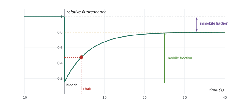
A simple model describes recovery as an exponential approach to a plateau. Fitting this model gives the half-time of recovery and the mobile fraction. For a circular bleached spot of radius w and free two-dimensional diffusion, a widely used approximation estimates the diffusion coefficient as D ≈ 0.224 w² / t½.
import numpy as np
from scipy.optimize import curve_fit
rng = np.random.default_rng(214)

# Simulated FRAP data for a membrane protein (normalized intensities)
F_initial = 1.0          # intensity before bleaching
t = np.linspace(0, 60, 61)            # seconds after the bleach
true = 0.15 + (0.80 - 0.15) * (1 - np.exp(-t / 6.0))
data = true + rng.normal(0, 0.015, t.size)

def model(t, F0, Finf, tau):
    return F0 + (Finf - F0) * (1 - np.exp(-t / tau))

(F0, Finf, tau), _ = curve_fit(model, t, data, p0=[0.1, 0.7, 5])
t_half = tau * np.log(2)
mobile = (Finf - F0) / (F_initial - F0)
w = 1.0                  # radius of bleached spot, um
D = 0.224 * w**2 / t_half
print(f"fitted F0 = {F0:.2f}, plateau = {Finf:.2f}, tau = {tau:.1f} s")
print(f"half-time of recovery = {t_half:.1f} s")
print(f"mobile fraction = {mobile:.2f}  (immobile {1 - mobile:.2f})")
print(f"estimated D = {D:.3f} um^2/s for a 1 um spot")fitted F0 = 0.16, plateau = 0.80, tau = 6.1 s half-time of recovery = 4.2 s mobile fraction = 0.77 (immobile 0.23) estimated D = 0.053 um^2/s for a 1 um spot
The fitted values say that about three-quarters of the labelled protein can move and that it diffuses with a coefficient of a few hundredths of a square micrometre per second, typical of membrane proteins. By comparison, a small soluble protein such as GFP diffuses in the cytoplasm at roughly 20 to 30 µm²/s, about a thousand times faster. Real FRAP analyses must account for diffusion during the bleach, binding and unbinding, and the shape of the bleached region, but the idea is the same.
Worked problem
From half-time to diffusion coefficient
A FRAP experiment on a cytosolic protein bleaches a spot of radius 2 µm. Fluorescence recovers with a half-time of 0.5 s. Estimate D and compare it with a membrane protein that recovers with a half-time of 20 s in the same spot.
Show solution
- D ≈ 0.224 w² / t½.
- Cytosolic protein: 0.224 × 4 / 0.5 ≈ 1.8 µm²/s.
- Membrane protein: 0.224 × 4 / 20 ≈ 0.045 µm²/s.
- The cytosolic protein moves about 40 times faster; its D is still below that of free GFP, suggesting it binds partners or is slowed by crowding.
Answer: About 1.8 µm²/s for the cytosolic protein and 0.045 µm²/s for the membrane protein.
Other quantitative approaches
Several other methods complement imaging. Flow cytometry measures the fluorescence of thousands of individual cells per second as they pass a laser in a stream, giving distributions rather than single images; lesson 12 uses it to measure DNA content through the cell cycle. Cell fractionation and proteomics, which identify and quantify thousands of proteins in each fraction by mass spectrometry, map which proteins belong to which organelle; large projects such as the Human Protein Atlas, which images the location of thousands of human proteins with antibodies, have shown that roughly half of human proteins are found in more than one compartment. Proximity labelling attaches an enzyme to a protein of interest that tags nearby proteins with biotin, revealing its neighbourhood. And single-cell sequencing measures gene expression in individual cells, revealing variation hidden in averages.
Good practice with images
Images are data and are subject to the same standards of honesty as any other data. Journals expect that adjustments to brightness and contrast are applied to the whole image and to controls equally, that no features are added, removed or moved, and that the original files are kept. Duplicated or manipulated images are a common reason for retraction of papers. Canadian researchers funded by the federal granting agencies follow the Tri-Agency Framework: Responsible Conduct of Research, while US researchers funded by federal agencies are covered by research misconduct rules that treat fabrication and falsification of images as misconduct.
Common mistakes
MistakeTwo proteins that colocalize in a fluorescence image must bind each other.
InsteadColocalization at light-microscope resolution means only that they are within about 200 nm; binding needs evidence such as FRET or biochemistry.
MistakeSuper-resolution microscopy breaks the laws of optics.
InsteadIt controls which molecules emit at any moment, so their positions can be found despite the diffraction limit.
MistakeA fluorescent tag never affects the protein.
InsteadA 27-kDa tag can block targeting signals or binding; tagged proteins must be tested for function.
MistakeIncomplete FRAP recovery means the experiment failed.
InsteadIncomplete recovery reveals an immobile fraction of molecules anchored to fixed structures.
MistakeBrightening only the interesting part of an image is acceptable if it shows the result better.
InsteadAdjustments must be applied equally to the whole image and to controls, and originals kept.
Summary and key terms
- Morphometry shows that internal membranes dwarf the plasma membrane and organelles fill nearly half the cell.
- Fluorescent proteins, self-labelling tags, dyes and biosensors make specific molecules and signals visible in living cells.
- Confocal, two-photon, light-sheet and TIRF microscopes reduce out-of-focus blur in different ways.
- STED, SIM and single-molecule localization microscopy reach 20–120 nm by controlling which molecules emit.
- Cryo-EM and cryo-electron tomography reveal molecular machines and their arrangement inside frozen cells.
- Quantitative image analysis requires background correction, unsaturated images, equal settings and many cells.
- Pearson’s coefficient measures colocalization; FRAP measures mobility, mobile fraction and diffusion coefficients.
- stereology
- Methods that estimate volumes and areas in three dimensions from measurements on thin sections.
- green fluorescent protein (GFP)
- A jellyfish protein that fluoresces green without cofactors, widely used as a genetic tag.
- biosensor
- An engineered fluorescent protein whose signal changes in response to a molecule or enzyme activity.
- confocal microscope
- A microscope that uses a pinhole to reject out-of-focus light, giving optical sections.
- TIRF microscopy
- Total internal reflection fluorescence, which excites only a thin layer next to the coverslip.
- super-resolution microscopy
- Fluorescence methods that resolve structures smaller than the diffraction limit.
- cryo-electron tomography
- Imaging a frozen specimen at many tilt angles to reconstruct it in three dimensions.
- colocalization
- The overlap of two labelled molecules in an image, often measured by Pearson’s coefficient.
- FRAP
- Fluorescence recovery after photobleaching, a method for measuring molecular mobility.
- mobile fraction
- The share of labelled molecules free to move into a bleached region.
Practice problems
Work each problem on paper first, then reveal the answer to check.
In a hepatocyte, roughly what percentage of total membrane is plasma membrane?
Show answer
About 2 per cent; internal membranes make up the rest.
Why was Chalfie’s 1994 experiment important?
Show answer
It showed that the GFP gene alone produces fluorescence in other organisms, so GFP can be used as a genetic tag.
What advantage does TIRF microscopy offer for studying vesicle fusion?
Show answer
It excites only about 100 nm into the cell, so events at the plasma membrane are seen against very low background.
Estimate the resolution of an objective with NA 1.4 using light of 560 nm.
Show answer
560 / (2 × 1.4) = 200 nm.
A single fluorophore spot has σ = 120 nm and 900 photons are detected. What is the ideal localization precision?
Show answer
120 / √900 = 4 nm.
What does cryo-ET show that single-particle cryo-EM does not?
Show answer
Molecular machines in their natural positions inside cells rather than averaged purified complexes.
Pearson’s r between two channels is 0.05. What does this suggest?
Show answer
No meaningful correlation: the two labels are not colocalized beyond chance.
In a FRAP experiment, intensity drops from 1.0 to 0.2 and recovers to 0.6. What is the mobile fraction?
Show answer
(0.6 − 0.2) / (1.0 − 0.2) = 0.5.
A 1.5-µm-radius spot recovers with t½ = 10 s. Estimate D.
Show answer
0.224 × 2.25 / 10 ≈ 0.05 µm²/s.
Name two rules for honest image processing.
Show answer
Apply adjustments to whole images and controls equally; never add, remove or move features; keep originals.
Lesson quiz · 5 questions
Score 60% or more to complete this lesson.
Create a free account to save your progress, take quizzes and earn a certificate.