
MBA-504 · Lesson 9 of 12 · 20 min
Regression in practice: dummies, interactions and diagnostics
Grace Mwangi's category includes Fairway's own-brand breakfast cereals, and the chain is reviewing how it prices and promotes them. Her analysts have two years of weekly data for every store: the shelf price, whether the product had an end-of-aisle display, the number of units sold and a handful of store characteristics. The merchandising director has two questions. How much do sales fall when the price goes up? And are displays worth the shelf space and labor they consume? A simple regression of units on price will not answer either question well, because displays and prices change together and because shoppers may respond to price differently when a product is on display. This lesson covers the tools that turn regression from a textbook exercise into a practical instrument.
Dummy variables
Many important explanatory variables are categories rather than numbers: whether a product is on display, the store format, the region, the day of the week, the quarter. Regression handles them through dummy variables, which take the value one when a condition holds and zero otherwise. In a model of units on price and a display dummy, the coefficient on the dummy is the average difference in units between display and non-display weeks at the same price. A category with several levels, such as four store formats, needs one dummy for each level except one, which becomes the baseline against which the others are compared. Including a dummy for every level, along with the intercept, makes the model impossible to estimate, a mistake known as the dummy variable trap.
Centering the price at three dollars, by subtracting three before fitting, makes the intercept meaningful: it is the predicted weekly units at a price of three dollars without a display. Fitting this model to 400 store-weeks of Grace's data gives an intercept of about 936 units, a price coefficient of about minus 162 units per dollar and a display coefficient of about 247 units. A display appears to add roughly 250 units a week, and each dollar on the price appears to cost about 160 units.
Interactions
The model above assumes that a display adds the same number of units at every price, and that price has the same effect with or without a display. Grace's analysts suspect otherwise. Shoppers who see a product at the end of an aisle are often browsing and comparing, and may be more sensitive to price. An interaction term, the product of two variables, allows the effect of one to depend on the level of the other. Adding display times centered price to the model lets the price slope differ between display and non-display weeks.
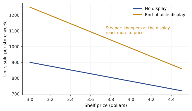
With the interaction included, the estimates are an intercept of about 909, a price slope of about minus 124 units per dollar without a display, a display effect of about 342 units at a price of three dollars, and an interaction of about minus 132. The price slope during display weeks is the sum of the two slope terms, about minus 256 units per dollar, roughly twice as steep. The display lift is largest at low prices and shrinks as the price rises: at 3.00 dollars it is about 342 units, but at 4.00 dollars it is about 342 minus 132, or 210 units.
# Dummy variable and interaction: price response with and without a display
import random, math
random.seed(9)
def solve(A, y):
    n = len(A); M = [row[:] + [v] for row, v in zip(A, y)]
    for i in range(n):
        p = max(range(i, n), key=lambda r: abs(M[r][i])); M[i], M[p] = M[p], M[i]
        for r in range(i + 1, n):
            f = M[r][i] / M[i][i]; M[r] = [a - f * b for a, b in zip(M[r], M[i])]
    x = [0.0] * n
    for i in reversed(range(n)):
        x[i] = (M[i][n] - sum(M[i][j] * x[j] for j in range(i + 1, n))) / M[i][i]
    return x
def ols(X, y):
    k = len(X[0])
    A = [[sum(r[i] * r[j] for r in X) for j in range(k)] for i in range(k)]
    return solve(A, [sum(r[i] * v for r, v in zip(X, y)) for i in range(k)])

rows = []
for _ in range(600):                                  # 600 store-weeks
    price = random.choice([2.99, 3.29, 3.49, 3.79, 3.99, 4.29, 4.49])
    display = 1 if random.random() < 0.3 else 0
    units = 900 - 120 * (price - 3) + display * (350 - 140 * (price - 3)) + random.gauss(0, 60)
    rows.append((price, display, units))
train, test = rows[:400], rows[400:]

def design(r, inter):
    p, d, _ = r
    return [1.0, p - 3, d, d * (p - 3)] if inter else [1.0, p - 3, d]
for inter in (False, True):
    b = ols([design(r, inter) for r in train], [r[2] for r in train])
    err = [r[2] - sum(c * x for c, x in zip(b, design(r, inter))) for r in test]
    rmse = math.sqrt(sum(e * e for e in err) / len(err))
    label = 'with interaction' if inter else 'no interaction  '
print(f"Model {label}: " + ", ".join(f"{c:7.1f}" for c in b) + f" holdout error {rmse:5.1f} units")Model no interaction : 936.2, -162.0, 246.5 holdout error 69.7 units Model with interaction: 908.8, -123.6, 342.3, -132.4 holdout error 59.9 units
The code fits both models on the first 400 store-weeks and tests them on the remaining 200, which the models have not seen. The holdout error, the typical size of prediction errors on new data, falls from about 70 units to about 60 when the interaction is included. That improvement on fresh data, rather than a higher R-squared on the data used for fitting, is the convincing evidence that the interaction is real and useful.
For the merchandising director, the interaction changes the advice. Displays work best when paired with a price cut, because shoppers at the display respond strongly to price. Putting the cereal on display at full price wastes much of the display's value. Grace recommends that displays run only during promotional price weeks, and that the promotional price be set using the steeper display slope.
Logs, percentages and elasticities
Business relationships are often better described in percentage terms than in units. A one-dollar price increase means something very different for a three-dollar box of cereal and a thirty-dollar bottle of olive oil. Taking natural logarithms of variables converts the model to percentage changes. When both the outcome and the explanatory variable are in logs, the slope is an elasticity: the percentage change in the outcome for a one percent change in the explanatory variable. This connects regression directly to the price elasticity of demand that Professor Varga introduced in MBA-502.
In Grace's linear model, the elasticity can be computed at a given point. At a price of 3.49 dollars without a display, predicted units are about 848 and the slope is about minus 124, so the elasticity is minus 124 times 3.49 divided by 848, about minus 0.51: demand is inelastic, and a modest price increase would raise revenue. With a display, at the same price, predicted units are about 1,126 and the slope about minus 256, giving an elasticity of about minus 0.79. Logs also help with right-skewed outcomes such as sales or income, because they tame the long tail and often turn a funnel-shaped residual plot into an even cloud.
| Model form | Interpretation of slope b1 |
|---|---|
| units = b0 + b1 x price | Change in units per one-dollar change in price |
| ln(units) = b0 + b1 x price | Approximate percentage change in units per one-dollar change, times 100 |
| units = b0 + b1 x ln(price) | Change in units per one percent change in price, times 100 |
| ln(units) = b0 + b1 x ln(price) | Percentage change in units per one percent change in price: the elasticity |
Curves and diminishing returns
Some relationships bend. Advertising usually shows diminishing returns: the first thousand dollars reaches new customers, while later spending mostly reaches people who have already seen the message. Adding a squared term to the model allows a curve; a positive coefficient on the linear term and a negative coefficient on the squared term describes a relationship that rises at a decreasing rate and eventually turns down. The peak occurs where the slope is zero, at minus b1 divided by twice b2. Curves should be used when theory or residual plots suggest them, not as a way to chase a better fit, and predictions should not be made beyond the range of the data, where a fitted curve can turn in implausible ways.
Diagnostics: what can go wrong
Dr. Zhou gives the cohort a checklist of diagnostics to run before trusting a regression. Plot the residuals against fitted values and each explanatory variable, looking for curves, funnels and clusters. Look for influential points, observations whose removal would change the coefficients substantially; a single store with a data error or an unusual event can tilt a line. Check whether residuals are correlated over time, which is common in weekly or monthly data and makes standard errors too small. Check whether the variance of residuals grows with the fitted values; if so, use logs or robust standard errors. And check for collinearity, which inflates standard errors when explanatory variables move together.
Influential points deserve particular care. Grace's analysts find that one store reported 9,000 units in a single week, ten times its usual level, because a school bought the cereal for a breakfast program. That one observation pulled the display coefficient up noticeably, because the store happened to have a display that week. The correct response is not to delete the point silently but to understand it: it is a genuine sale, but it represents a different kind of demand from household shopping, so the analysts exclude it from the price model, record the exclusion and report sales to institutions separately.
Overfitting and validation
Adding variables to a regression never reduces R-squared on the data used for fitting, so a model can always be made to look better by adding more terms. Eventually it begins to fit the noise in that particular sample rather than the underlying pattern, a problem called overfitting. An overfitted model predicts the past well and the future badly. The defense is to test models on data they were not fitted to. A simple approach is the holdout split used above: fit on one part of the data and measure prediction error on the rest. Cross-validation repeats this many times with different splits and averages the results. Adjusted R-squared, which penalizes extra variables, offers a rough guide when data are too scarce to split.
The same principle underlies machine learning, which many of the cohort's companies now use. Methods such as random forests and gradient boosting can capture interactions and curves automatically and often predict better than a hand-built regression. Their weakness is interpretability: they are good at answering what will happen, less good at explaining why or at estimating the effect of a decision such as a price change, because they learn whatever correlations help prediction, including confounded ones. Dr. Zhou's advice is to match the tool to the question. For forecasting demand, use whatever predicts best on held-out data. For deciding what a price change will do, use a model, or better an experiment, designed to estimate that effect.
Yes-or-no outcomes
Many business outcomes are binary: a customer renews or does not, a loan defaults or does not, a patient is readmitted or is not. A linear regression on a zero-one outcome can produce predicted probabilities below zero or above one. Logistic regression models the log of the odds instead, which keeps predictions between zero and one. Its coefficients are interpreted through odds ratios: a coefficient of 0.4 on a variable means that a one-unit increase multiplies the odds of the outcome by e to the 0.4, about 1.5. Leo's team uses logistic regression to estimate each customer's probability of renewal from usage, support tickets and contract length, and ranks accounts for attention by expected revenue at risk.
Worked problem
Reading Leo's renewal model
Kestrel's logistic regression for renewal includes active users per license (a share from 0 to 1), the number of support tickets last quarter and a dummy for an annual rather than monthly contract. The coefficients are: intercept minus 0.8, active share 3.0, tickets minus 0.15, annual 0.9. Estimate the renewal probability for a monthly customer with an active share of 0.6 and 4 tickets.
Show solution
- Compute the log-odds: minus 0.8 + 3.0 x 0.6 minus 0.15 x 4 + 0.9 x 0 = minus 0.8 + 1.8 minus 0.6 = 0.4.
- Convert to odds: e to the 0.4, about 1.49.
- Convert to probability: 1.49 divided by (1 + 1.49), about 0.60.
- Compare: an otherwise identical annual customer has log-odds 1.3, odds about 3.67 and probability about 0.79.
Answer: The monthly customer has about a 60 percent chance of renewing. The annual-contract dummy multiplies the odds by e to the 0.9, about 2.5, although this is an association: customers who choose annual contracts may already be more committed, so the model alone does not show that moving customers to annual contracts would raise renewals by that much.
Common mistakes
MistakeInclude a dummy for every category level.
InsteadUse one fewer dummy than levels; the omitted level is the baseline.
MistakeA display adds the same number of units at any price.
InsteadTest an interaction; effects often depend on other variables.
MistakeA model with more variables and higher R-squared is better.
InsteadJudge models by prediction error on held-out data to avoid overfitting.
MistakeA predictive model shows what a decision will do.
InsteadPrediction and causal effect differ; use a design that estimates the effect of the decision.
Summary and key terms
- Dummy variables bring categories into regression; use one fewer than the number of levels.
- Interaction terms let the effect of one variable depend on another.
- In a log-log model the slope is an elasticity; logs also tame skewed outcomes.
- Check residuals, influential points, correlated errors and collinearity before trusting a model.
- Validate on held-out data and use logistic regression for yes-or-no outcomes.
- Dummy variable
- A variable equal to one when a condition holds and zero otherwise.
- Interaction term
- The product of two variables, allowing the effect of one to depend on the other.
- Elasticity
- The percentage change in one variable for a one percent change in another.
- Influential point
- An observation whose removal would substantially change the fitted model.
- Overfitting
- Fitting noise in the sample so that the model predicts new data poorly.
- Logistic regression
- A model for yes-or-no outcomes that predicts probabilities through the log-odds.
Practice problems
Work each problem on paper first, then reveal the answer to check.
A model of weekly sales includes dummies for Tuesday to Sunday. What does the coefficient on the Saturday dummy mean?
Show answer
The average difference in sales between Saturday and Monday, the omitted baseline day, holding other variables constant.
In a log-log regression of units on price, the price coefficient is minus 1.8. What happens to units if price rises 5 percent?
Show answer
Units fall by about 1.8 x 5 = 9 percent; demand is elastic.
A model with an interaction gives units = 900 minus 120 x (price minus 3) + 340 x display minus 130 x display x (price minus 3). What is the display lift at a price of 3.50 dollars?
Show answer
340 minus 130 x 0.5 = 275 units.
A logistic regression coefficient on a loyalty-member dummy is 0.7. How does membership change the odds of purchase?
Show answer
It multiplies the odds by e to the 0.7, about 2.0, so members have roughly double the odds of purchase, holding other variables constant.
Lesson quiz · 5 questions
Score 60% or more to complete this lesson.
Create a free account to save your progress, take quizzes and earn a certificate.