
MBA-504 · Lesson 2 of 12 · 22 min
Describing data: distributions, summaries and visualization
Grace Mwangi opens the second weekend with a problem from Fairway Grocers. The chain's executive team has set a goal to raise the average basket, the amount a customer spends on a single shopping trip, by five percent over the next year. Each of Grace's forty store managers receives a weekly report showing their store's average basket against the target. Several managers have complained that the number jumps around for no reason they can see, and one store manager in a suburban location has been praised two weeks running because a catering company placed two very large orders. Grace suspects the measure is misleading, but she cannot explain why to her vice-president. Dr. Zhou says the answer lies in the shape of the data, and that describing data well is the most underrated skill in management.
Types of data
Before summarizing anything, it helps to know what kind of variable is being measured, because the type determines which summaries and charts make sense. Categorical variables place each observation in a group: the store, the payment method, the product category or whether a customer holds a loyalty card. Some categorical variables have a natural order, such as a satisfaction rating from very dissatisfied to very satisfied, and are called ordinal. Numerical variables are measured on a scale where differences have meaning: the basket amount in dollars, the number of items, the minutes a patient waits. Numerical variables can be discrete, taking whole-number values such as items in a basket, or continuous, such as time or weight.
The distinction matters in practice. An average of a categorical code is meaningless: if Fairway codes payment as 1 for cash, 2 for debit and 3 for credit, an average of 2.3 says nothing. Ordinal ratings are often averaged anyway, and the result can be useful as a rough summary, but managers should remember that the gap between very dissatisfied and dissatisfied is not necessarily the same as the gap between satisfied and very satisfied. Reporting the share of customers in the top two boxes, or the full distribution of ratings, is often clearer than an average of codes.
The shape of a distribution
A distribution shows how often each value, or range of values, occurs. For a numerical variable the basic picture is a histogram, which groups values into bins and draws a bar for the number of observations in each. Grace pulls one month of transactions for a single store, about five thousand baskets, and draws the histogram. Most baskets fall between twenty and seventy dollars, but a long tail stretches to the right: some customers spend two hundred dollars or more on a weekly family shop or a party. A distribution with a long tail on the right is called right-skewed, and it is the normal shape for money amounts, waiting times, incomes, claim sizes and many other business quantities that cannot fall below zero but can be very large.
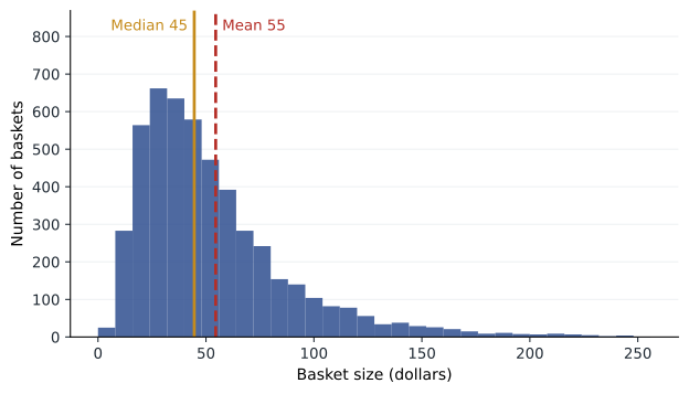
In a right-skewed distribution the mean, the arithmetic average, is pulled toward the tail by the large values. For Grace's store the mean basket is about fifty-five dollars while the median, the middle value when baskets are sorted, is about forty-five dollars. Neither number is wrong; they answer different questions. The mean is what matters for revenue, because total sales equal the mean basket times the number of baskets. The median describes the typical customer. If Fairway wants to understand what most shoppers experience, the median is the better guide; if it wants to forecast revenue, the mean is the one it needs.
The skew also explains the suburban store's two good weeks. A mean is sensitive to a few extreme values, and two catering orders of several thousand dollars each were enough to lift that store's weekly average basket above the target even though nothing about its ordinary customers had changed. The median would barely have moved. A manager who rewards changes in the mean of a skewed variable is partly rewarding luck in the tail.
Measuring spread
A summary of the center of a distribution is incomplete without a summary of its spread. Two stores with the same median basket can be very different businesses if one serves a narrow band of commuters buying lunch and the other serves families whose spending ranges from a single item to a full trolley. The most common measure of spread is the standard deviation, which is roughly the typical distance of an observation from the mean. It is calculated by squaring each deviation from the mean, averaging the squares (dividing by one less than the number of observations for a sample) and taking the square root.
Like the mean, the standard deviation is sensitive to extreme values, so for skewed data managers often prefer percentiles. The 25th percentile is the value below which a quarter of observations fall, and the 75th percentile the value below which three-quarters fall. The distance between them, the interquartile range, covers the middle half of the data. For Grace's store the quartiles are about twenty-nine and sixty-seven dollars, so half of all baskets fall in that range, and the 90th percentile is about a hundred dollars. Percentiles are also how many service standards are written: a hospital might commit that 90 percent of emergency patients are assessed within a set time, which is a statement about the 90th percentile, not the average.
# Summaries of a right-skewed variable using only the standard library
import random, statistics
random.seed(42)
baskets = [random.lognormvariate(3.8, 0.65) for _ in range(5000)]   # one month of baskets at one store

q = statistics.quantiles(baskets, n=100)          # 99 cut points: q[24] is the 25th percentile
print(f"Mean     {statistics.mean(baskets):6.1f}")
print(f"Median   {statistics.median(baskets):6.1f}")
print(f"Std dev  {statistics.stdev(baskets):6.1f}")
print(f"P25      {q[24]:6.1f}   P75 {q[74]:6.1f}   IQR {q[74] - q[24]:5.1f}")
print(f"P90      {q[89]:6.1f}")

# Two very large catering orders added to a week of about 1,200 baskets
week = baskets[:1200]
with_orders = week + [4200.0, 3800.0]
print(f"Weekly mean without orders {statistics.mean(week):6.1f}, with orders {statistics.mean(with_orders):6.1f}")
print(f"Weekly median without orders {statistics.median(week):6.1f}, with orders {statistics.median(with_orders):6.1f}")Mean 55.3 Median 44.3 Std dev 40.3 P25 28.7 P75 69.0 IQR 40.2 P90 103.6 Weekly mean without orders 55.6, with orders 62.1 Weekly median without orders 44.6, with orders 44.7
The output shows the gap between mean and median, the wide interquartile range and the effect of two large orders. Two baskets out of more than a thousand lift the weekly mean by several dollars, comfortably more than the five percent target, while the median moves by a few cents. Grace now has a concrete way to explain to her vice-president why the weekly league table rewards the wrong stores.
Outliers: errors, exceptions or the main story
An outlier is an observation far from the rest. The first question is whether it is an error. A basket of forty thousand dollars is probably a scanning mistake or a test transaction; a negative wait time is a data-entry error. Errors should be corrected or removed, and the rule used should be written down. The second question is whether the outlier belongs to a different population. The catering orders are genuine sales, but they come from business customers, not households, and analyzing them together hides two different patterns. Fairway's better approach is to report household baskets and business orders separately.
The third possibility is that the outliers are the story. In insurance, a small number of very large claims drives most of the cost. In software, a few large customers often provide most of the revenue. At Lakeview Health, Hana notes that around five percent of patients account for a large share of emergency visits, a pattern health systems in many countries have reported. Removing them as outliers would make the data look tidier and the analysis useless. Dr. Zhou's rule is never to delete an observation simply because it is inconvenient, and always to report how many were removed and why.
Comparing groups
Managers rarely care about one distribution on its own; they want to compare stores, regions, shifts, products or periods. The boxplot is designed for this. Each box spans the interquartile range, a line inside marks the median, whiskers extend to the most extreme values within a set distance of the box, and points beyond the whiskers are plotted individually. Placing boxplots side by side shows differences in typical value, spread and skew at a glance.
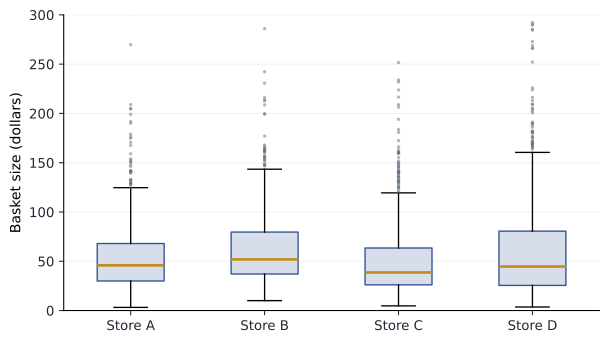
Grace's boxplots for four stores show that Store B has the highest median, but Store D has the widest spread and the longest tail, consistent with a location that serves both small top-up shops and very large family shops. A target expressed as a single average treats these stores as if they were alike. Grace considers two alternatives: tracking the median basket for households, which reflects ordinary customer behavior, and tracking the share of baskets above a threshold such as seventy-five dollars, which shows whether more customers are doing a full shop at Fairway rather than splitting it with a competitor.
Choosing the right chart
Most business charts should answer a single question, and the question determines the form. To compare amounts across categories, a bar chart with a common baseline at zero is hard to beat. To show change over time, a line chart with time on the horizontal axis is the natural choice. To show the relationship between two numerical variables, such as price and units sold, a scatter plot reveals patterns, clusters and outliers that a table hides. To show a distribution, a histogram or boxplot. Pie charts work only when there are a few categories that make up a whole and the differences are large; people judge angles and areas far less accurately than lengths along a common scale, a finding that goes back to experiments by William Cleveland and Robert McGill in the 1980s.
| Question | Good chart | Common mistake |
|---|---|---|
| How do amounts compare across stores? | Bar chart sorted by value, axis from zero | Bars in alphabetical order, truncated axis |
| How has a measure changed over time? | Line chart with consistent time intervals | Bar chart of irregular periods |
| Are two measures related? | Scatter plot, one point per unit | Two lines on separate axes |
| How are values spread? | Histogram or boxplot | A single average with no spread |
| What share does each part take? | Stacked bar or a few labeled bars | Pie with ten slices |
How charts mislead
Charts can mislead even when every number is correct. A bar chart whose vertical axis starts at 95 rather than zero can make a two percent difference look like a doubling. A line chart with two vertical axes can make any two series appear to move together, because the analyst chooses the scales. Charts of cumulative totals always rise, which can hide a slowdown. Percentages without the underlying counts can turn a change from two complaints to four into a headline about a 100 percent increase. Area and three-dimensional effects distort comparisons. And choosing the start and end dates of a time series can create or erase a trend.
Leo admits that his company's investor presentations have used most of these tricks at one time or another, usually without intending to deceive. Dr. Zhou suggests a test before any chart goes to a board: could a skeptical reader, given the same data, reasonably draw a different conclusion from a fairly drawn version? If so, redraw it. For line charts of measures such as defect rates or wait times, the axis need not start at zero, because the question is about change, but the scale should be stated and the range should be wide enough to show normal variation.
Dashboards that support decisions
Dashboards are the most common way managers meet data, and most of them suffer from the problem Dr. Zhou showed on the first evening: too many metrics, none tied to a decision. A useful dashboard is built backwards from the decisions it supports. For each metric, the designer should be able to say who looks at it, how often, what normal variation looks like and what action follows when it moves outside that range. Metrics that no one acts on should be removed. Showing a short history and a band of normal variation next to each number, rather than a single colored tile, helps people distinguish signal from noise.
Grace redesigns the store report around four measures: median household basket, share of household baskets over seventy-five dollars, number of household transactions and business orders reported separately. Each is shown as a twelve-week line with a shaded band marking the range covered by the store's own previous year of weekly values. Store managers are asked to explain only movements outside the band. Her vice-president agrees to replace the weekly league table with a quarterly review, which smooths out much of the noise.
Worked problem
Choosing a summary for Hana's wait times
Lakeview's emergency department records the time from arrival to first assessment by a physician or nurse practitioner. In one month, 4,000 patients have a mean wait of 74 minutes and a median wait of 52 minutes; the 90th percentile is 165 minutes. The board wants a single headline number.
Show solution
- Recognize the shape: the mean is well above the median, so the distribution is right-skewed with a long tail of very long waits.
- Identify the decision: the board is concerned with patients who wait far too long, which is a tail problem.
- Choose the summary: the 90th percentile directly measures the experience of the longest-waiting tenth of patients, and many health systems set targets in this form.
- Add context: report the median alongside it, and show both as monthly lines with a band of normal variation.
Answer: Hana recommends the 90th percentile wait, currently 165 minutes, as the headline measure, with the median as a companion. A reduction in the mean could be achieved by speeding up already short waits, while the 90th percentile improves only if the longest waits come down.
Common mistakes
MistakeThe mean is always the best summary of a typical value.
InsteadFor skewed data the median better describes the typical case; the mean is needed for totals.
MistakeOutliers should be removed to clean the data.
InsteadCheck whether they are errors, a different population or the main story, and report what was removed.
MistakeA chart is honest if the numbers are correct.
InsteadAxis choices, dual scales, date ranges and percentages without counts can mislead with correct numbers.
MistakeMore dashboard metrics give better oversight.
InsteadEach metric should have an owner, a normal range and an action; others add noise.
Summary and key terms
- Identify whether a variable is categorical, ordinal or numerical before choosing summaries.
- Money amounts, waits and claims are usually right-skewed, so the mean exceeds the median.
- Use the standard deviation, interquartile range and percentiles to describe spread; percentiles suit skewed data and service targets.
- Compare groups with side-by-side boxplots and choose charts from the question they answer.
- Build dashboards backwards from decisions, showing history and normal variation.
- Distribution
- The pattern of how often each value or range of values occurs.
- Right-skewed
- A distribution with a long tail of large values, which pulls the mean above the median.
- Median
- The middle value when observations are sorted.
- Standard deviation
- A measure of the typical distance of observations from the mean.
- Interquartile range
- The distance between the 25th and 75th percentiles, covering the middle half of the data.
- Boxplot
- A chart showing the median, quartiles and extreme values of a distribution.
Practice problems
Work each problem on paper first, then reveal the answer to check.
Monthly incomes of a company's customers have a mean of 6,800 dollars and a median of 5,100 dollars. What does this tell you about the shape of the distribution?
Show answer
The distribution is right-skewed: a minority of high incomes pulls the mean above the median.
Why might a call center set a target for the 80th percentile of answer time rather than the mean?
Show answer
The target then focuses on the callers who wait longest; a mean can improve while many callers still wait far too long.
A chart shows customer satisfaction rising from 81 to 84 percent with the axis running from 80 to 85. What would you change?
Show answer
Label the axis clearly and widen it or start it lower, and show the sample size or a range of normal variation so readers can judge whether a three-point change is meaningful.
A data file of delivery times contains three values of minus 15 minutes. What should an analyst do?
Show answer
Treat them as errors, investigate the cause, correct or remove them, and record the rule used and the number removed.
Lesson quiz · 5 questions
Score 60% or more to complete this lesson.
Create a free account to save your progress, take quizzes and earn a certificate.