
MBA-504 · Lesson 12 of 12 · 23 min
Capstone: a data-driven recommendation for Cedarline Outdoor
The final weekend of Data Analysis for Managers returns to Cedarline Outdoor, the apparel and equipment company the cohort has followed since MBA-501. Its story is familiar by now. Revenue grew from 312 million dollars in fiscal 2022 to 468 million in fiscal 2026, but inventory more than doubled, from 58 million to 128 million, and the cash conversion cycle stretched from 99 to 177 days. Return on invested capital of about 8 percent sits below the company's estimated 9 percent cost of capital, so growth has been destroying value. In MBA-502 the cohort used price elasticity to rethink pricing on the Ridgeline jacket; in MBA-503 it diagnosed the leadership and culture behind the company's problems. Now Cedarline's chief operating officer has asked the Lakeshore cohort in Chicago for a recommendation grounded in data: how should the company use analytics to restore value creation over the next eighteen months?
Dr. Zhou divides the five managers into a single consulting team and gives them three weeks of Cedarline data: online and store transactions, weekly sales by product and region, inventory positions, buying plans, a recent website experiment and the results of a customer survey. Their task is to apply the whole course: start with the decision, describe the data honestly, quantify uncertainty, separate correlation from causation, model what drives outcomes, forecast, and structure the final choices as decisions under uncertainty. This lesson follows their work.
Step 1: Write the decision brief
The team's first draft brief is too broad: improve Cedarline's performance with analytics. Using Dr. Zhou's template from lesson 1, they narrow it to three decisions the chief operating officer actually controls in the next budget cycle. First, whether to change the free-shipping threshold for online orders, which affects both revenue and costs. Second, how to set prices and promotions for the core outerwear range, which accounts for about a third of revenue and most of the excess inventory. Third, whether to replace the current buying process, in which category managers set seasonal order quantities largely by judgment, with a statistical forecasting system. The measure of success is economic profit, operating profit after a charge for the capital tied up in inventory, with a deadline of the spring buying cycle.
| Decision | Options | Measure | Evidence needed |
|---|---|---|---|
| Free-shipping threshold | Keep 150 dollars; lower to 100; lower to 75 | Gross margin after shipping per visitor | Randomized website test |
| Outerwear pricing and promotion | Current calendar; fewer, deeper promotions; targeted markdowns | Gross margin and end-of-season inventory | Demand model from weekly sales |
| Buying process | Keep judgmental buying; roll out forecasting system; pilot first | Forecast error, inventory and stockouts | Backtest and pilot results |
Step 2: Describe the data honestly
Before testing anything, the team describes what the data contain. Online order values are strongly right-skewed: the median order is about 96 dollars and the mean about 131, pulled up by customers buying tents, sleeping bags and multiple jackets. About 14 percent of online orders are returned, but returns are concentrated in apparel and among customers who order several sizes of the same item. Grace notices that the company's weekly dashboard reports average order value, which, as she learned in lesson 2, is dominated by a few large orders and moves with noise. The team recommends reporting the median order, the share of orders above the free-shipping threshold and return-adjusted margin instead.
Hana checks the data-generating process. The survey of 3,200 customers was sent only to loyalty members, who make up about 40 percent of customers and spend more than average, so its finding that 71 percent of respondents rate Cedarline's quality highly cannot be read as a measure of all customers. Daniel finds that the inventory system records markdowns only when items are sold, so goods that are sitting in warehouses well past their season still appear at full cost, overstating the value of the inventory and understating the problem.
Step 3: Test the free-shipping threshold
Cedarline's marketing team had already run a three-arm website experiment for four weeks, randomly assigning about 60,000 visitors to each of three free-shipping thresholds: the current 150 dollars, 100 dollars and 75 dollars. Leo, drawing on lesson 5, insists on looking at the right metric. Conversion rate rose in both test arms, but lower thresholds also mean Cedarline pays for shipping on more orders. The primary metric, chosen before the test began, was gross margin after shipping costs per visitor, which captures both effects.
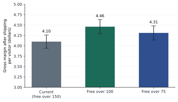
The 100-dollar threshold raised margin per visitor from 4.10 to 4.46 dollars, a lift of 36 cents with a z statistic of about 3.0 and a p-value of about 0.0025. Because the team made two comparisons against the current threshold, they apply the Bonferroni correction from lesson 6 and require a p-value below 0.025; the 100-dollar result passes comfortably. The 75-dollar threshold produced a smaller lift of 21 cents that is not statistically distinguishable from zero after correction. The team checks the traffic split for a sample ratio mismatch and finds none, and checks a guardrail metric, the return rate, which did not rise.
At the point estimate, with about six million online visitors a year, the 100-dollar threshold would add about 2.2 million dollars of annual gross margin. Mindful of the winner's curse, the team discounts this and recommends rolling out the 100-dollar threshold to 90 percent of visitors while keeping a 10 percent holdout at the old threshold for a further quarter, which will measure the real effect at scale and catch any longer-term change in customer behavior.
Step 4: Model outerwear demand
For outerwear, the team cannot run a clean experiment in time for the spring decision, so it builds a regression model from three years of weekly sales across 18 jacket styles and six regions, using the techniques of lessons 8 and 9. The outcome is the logarithm of weekly units; the explanatory variables include the logarithm of the selling price, dummies for promotion weeks, style, region and week of the season, and the deviation of regional temperature from normal. An interaction between promotion and the logarithm of price tests whether promotions change price sensitivity.
The estimated price elasticity outside promotions is about minus 2.4, with a 95 percent interval from about minus 2.9 to minus 1.9, consistent with the estimate of minus 2.43 for the Ridgeline jacket that the cohort used in MBA-502. Promotion weeks show a sharp lift in sales but also a significantly steeper price response, so most of the promotion effect comes from the price cut itself rather than the promotional signage. Colder-than-normal weeks raise sales strongly, which explains part of why the promotion calendar looked successful in a cold year. Daniel points out that this is confounding in action: the past promotion calendar was planned around expected cold snaps, so a naive comparison of promotion and non-promotion weeks credits the promotions with the weather's effect.
The model fits well, and on a holdout of the most recent season it predicts weekly units with a mean absolute percentage error of about 18 percent at the style-region level, far better than the buying plans. Its residual plots show no strong pattern. The team is careful about what the model can and cannot claim. Price varied mainly through planned promotions and markdowns, which were themselves chosen partly in response to slow sales, so the elasticity estimate could still be biased. They recommend a series of small randomized price tests across regions next autumn to confirm it, as lesson 7 suggested.
Step 5: Forecast to buy better
The largest prize is inventory. Owen leads a backtest of a statistical forecasting approach, using seasonal indices, trend and the demand model, against the category managers' historical buying plans for the past two seasons. Measured as a share of actual demand, the buyers' plans had an average absolute error of about 34 percent at the style level, with a strong upward bias: they bought too much far more often than too little. The statistical forecasts had an average error of about 24 percent and almost no bias. Combining the statistical forecast with buyer adjustments, but only where buyers recorded specific information such as a new product launch or a confirmed wholesale order, reduced the error slightly further, echoing the evidence on judgmental adjustment from lesson 10.
Lower forecast error translates directly into lower safety stock, the inventory held to cover uncertainty. In standard inventory models, safety stock is proportional to the standard deviation of forecast error over the replenishment lead time, so a reduction in error from 34 to 24 percent of demand cuts the safety stock needed for the same service level by about 29 percent. The team estimates, with a wide range, that better forecasting and removing the upward bias could reduce Cedarline's inventory by 15 to 25 million dollars over two seasons without increasing stockouts, shortening the cash conversion cycle by roughly 20 to 35 days.
# Cedarline capstone: threshold test, forecast error and a pilot decision
import math
from statistics import NormalDist

# 1. Free-shipping threshold test: gross margin after shipping per visitor (dollars)
arms = {'Current (150)': (4.10, 0.16), 'Over 100': (4.46, 0.17), 'Over 75': (4.31, 0.17)}   # mean, 95% half-width
base_mean, base_half = arms['Current (150)']
for name in ('Over 100', 'Over 75'):
    m, h = arms[name]
    se = math.sqrt((h / 1.96) ** 2 + (base_half / 1.96) ** 2)
    z = (m - base_mean) / se
    p = 2 * (1 - NormalDist().cdf(abs(z)))
    print(f"{name:9s} lift {m - base_mean:+.2f} per visitor, z = {z:.2f}, p = {p:.4f}, passes Bonferroni (0.025): {p < 0.025}")
visitors = 6_000_000
print(f"Annual value of the 100 threshold at the point estimate: {0.36 * visitors / 1e6:.2f} million")

# 2. Safety stock scales with forecast error: cutting error from 34% to 24% of weekly demand
z95, weekly, lead_weeks = 1.645, 1000, 9
for err in (0.34, 0.24):
    ss = z95 * err * weekly * math.sqrt(lead_weeks)
    print(f"Forecast error {err:.0%}: safety stock about {ss:,.0f} units per 1,000 units of weekly demand")
print(f"Reduction: {1 - 0.24 / 0.34:.0%}")

# 3. Roll out a new forecasting system now, or pilot it first (million dollars)
p_good = 0.6
now = p_good * 12 + (1 - p_good) * (-10)
pos_if_good, pos_if_poor, pilot_cost, good_later = 0.85, 0.25, 0.8, 11
p_pos = pos_if_good * p_good + pos_if_poor * (1 - p_good)
g_pos = pos_if_good * p_good / p_pos
g_neg = (1 - pos_if_good) * p_good / (1 - p_pos)
ev_pos = max(0, g_pos * good_later + (1 - g_pos) * (-10))
ev_neg = max(0, g_neg * good_later + (1 - g_neg) * (-10))
pilot = p_pos * ev_pos + (1 - p_pos) * ev_neg - pilot_cost
print(f"Roll out now EV {now:.2f}; pilot first EV {pilot:.2f} (P positive {p_pos:.2f}, P good | positive {g_pos:.2f})")Over 100 lift +0.36 per visitor, z = 3.02, p = 0.0025, passes Bonferroni (0.025): True Over 75 lift +0.21 per visitor, z = 1.76, p = 0.0779, passes Bonferroni (0.025): False Annual value of the 100 threshold at the point estimate: 2.16 million Forecast error 34%: safety stock about 1,678 units per 1,000 units of weekly demand Forecast error 24%: safety stock about 1,184 units per 1,000 units of weekly demand Reduction: 29% Roll out now EV 3.20; pilot first EV 3.81 (P positive 0.61, P good | positive 0.84)
Step 6: Structure the rollout decision
Replacing the buying process is not risk-free. The forecasting system will cost money to implement, buyers may resist it, and the backtest may flatter it, since it was tuned on the same seasons it was tested on. The team builds a decision tree, using lesson 11. A full rollout now would yield a net present value of about 12 million dollars if the system performs well in live use, which the team estimates at 60 percent, and a loss of about 10 million if it performs poorly and disrupts buying for a season, for an expected value of 3.2 million.
The alternative is a one-season pilot in two categories, costing 0.8 million and delaying the full benefits, so the payoff if the system works falls to about 11 million. The pilot is informative but imperfect: the team estimates that it would show good results 85 percent of the time if the system works and 25 percent of the time if it does not. Rolling back the tree gives an expected value of about 3.8 million for piloting first, against 3.2 million for rolling out now. The value of the pilot lies in avoiding the 10 million loss: after a poor pilot result, the probability that the system works falls to about 23 percent, and Cedarline would not proceed. The team adds a sensitivity analysis showing that the pilot remains the better choice unless the probability that the system works is above about 66 percent, so the recommendation is sensitive to that estimate and the team flags it for discussion.
Step 7: Write the recommendation
Dr. Zhou insists that the recommendation fit on two pages and lead with decisions, not methods. The team's memo to the chief operating officer makes four recommendations. Lower the free-shipping threshold to 100 dollars now, with a 10 percent holdout for a quarter to confirm the effect. Cut the number of outerwear promotion weeks and shift markdown decisions to a model-based process that accounts for weather, while running randomized regional price tests to confirm the elasticity. Pilot the statistical forecasting system in two categories this spring, with a decision on full rollout before the autumn buying cycle based on pre-agreed measures of forecast error, bias and stockouts. And replace the weekly dashboard's average order value with median order value, margin per visitor and inventory weeks of supply, each shown with a band of normal variation.
The memo states its uncertainties plainly. The threshold gain is estimated within a range and may shrink at scale. The elasticity rests on observational data. The inventory reduction is a range, not a promise. Each recommendation includes the measure that will show whether it is working and the point at which the company should change course. Leo observes that this is the opposite of the confident slide decks he used to present, and that it is far more persuasive to a skeptical board, because every claim can be checked.
Using data responsibly
Several of the team's ideas involve customer data, and Hana raises the question of how it should be used. Personalized pricing based on browsing history might raise short-term margin, but it risks customer anger if discovered and may conflict with privacy and consumer protection law. The team limits its recommendations to aggregate analysis and randomized tests of prices that all visitors in a region see equally, and recommends that the company's privacy officer review the data used in the forecasting system. Dr. Zhou closes the course by returning to her opening slide: the point of all this work is not more data or more dashboards, but better decisions, made with honest awareness of what the data can and cannot say.
Worked problem
Estimating the value of the inventory reduction
Cedarline's inventory is 128 million dollars and its cost of capital is about 9 percent. The team estimates that better forecasting could reduce inventory by 20 million dollars, the middle of its range, and that holding costs other than capital, such as storage, insurance, obsolescence and handling, amount to about 12 percent of inventory value a year.
Show solution
- Capital charge saved: 9 percent of 20 million = 1.8 million a year.
- Other holding costs saved: 12 percent of 20 million = 2.4 million a year.
- Total annual benefit: 1.8 + 2.4 = 4.2 million, plus a one-time release of 20 million of cash.
- Effect on the cash conversion cycle: with cost of goods sold of about 260 million a year, days of inventory fall by 20 / 260 x 365, about 28 days.
Answer: A 20 million reduction in inventory would save about 4.2 million a year and release 20 million of cash, cutting the cash conversion cycle by about four weeks. Together with the shipping-threshold gain, this would move a meaningful part of the way toward closing the gap between Cedarline's return on capital and its cost of capital.
Common mistakes
MistakeA capstone recommendation should show every analysis performed.
InsteadLead with decisions and the evidence behind them; put methods in an appendix.
MistakeAn experiment result can be rolled out at the measured effect.
InsteadExpect shrinkage; keep a holdout to measure the effect at scale.
MistakeA well-fitting demand model shows the effect of price changes.
InsteadObservational price variation may be confounded; confirm with randomized tests.
MistakeA promising new system should be rolled out at once.
InsteadWhen failure is costly and a pilot is informative, piloting first can have higher expected value.
Summary and key terms
- Start from a decision brief that names decisions, options, measures and deadlines.
- Describe data and check how they were generated before testing or modeling.
- Use randomized tests with pre-chosen metrics and multiple-comparison corrections where possible.
- Model and forecast with honest uncertainty, watching for confounding such as weather.
- Structure rollouts as decisions under uncertainty and present recommendations with ranges and tracking measures.
- Economic profit
- Operating profit after a charge for the capital employed.
- Holdout group
- A randomly chosen group kept on the old policy after rollout to measure the effect at scale.
- Safety stock
- Inventory held to protect against forecast error and supply variability.
- Backtest
- Testing a forecasting or decision method on past data it was not fitted to.
- Margin per visitor
- Gross margin after variable costs divided by the number of website visitors.
- Pilot
- A limited trial of a change used to gather information before a full commitment.
Practice problems
Work each problem on paper first, then reveal the answer to check.
Why did the team choose margin per visitor rather than conversion rate as the primary metric for the threshold test?
Show answer
Lower thresholds raise conversion but also increase shipping costs; margin per visitor captures both effects and ties to profit.
The 75-dollar threshold had a p-value of about 0.078. Why did the team not recommend it?
Show answer
It did not reach significance even before correction, and with two comparisons the Bonferroni threshold was 0.025; its gain was smaller and uncertain.
How could weather confound an analysis of outerwear promotions?
Show answer
Promotions were scheduled around expected cold weeks, and cold weather raises sales, so a naive comparison credits promotions with part of the weather effect.
If forecast error falls from 30 to 21 percent of demand, by roughly how much does the required safety stock fall?
Show answer
Safety stock is proportional to forecast error, so it falls by about 30 percent.
Lesson quiz · 5 questions
Score 60% or more to complete this lesson.
Create a free account to save your progress, take quizzes and earn a certificate.