
MBA-504 · Lesson 3 of 12 · 21 min
Probability, uncertainty and base rates
Owen Tremblay brings a puzzle to the third session. Prairie Ridge Energy installed a vibration-monitoring system on a group of wind turbines last year, and the vendor's brochure says the system detects 90 percent of gearbox problems before they cause a failure, with a false alarm rate of only five percent. The operations team now receives an alarm and must decide whether to shut a turbine down for an inspection that costs a day of lost generation and a crane crew. The site manager assumes that an alarm means a 90 percent chance of a failing gearbox. Owen's instinct is that the real figure is much lower, but he cannot say why. Dr. Zhou tells him that the missing ingredient is the base rate, and that this single idea prevents more expensive mistakes than any other in the course.
What probability means to a manager
A probability is a number between zero and one that expresses how likely an event is. There are two complementary ways to think about it. The frequency view treats probability as the long-run share of times an event happens in repeated trials: if two percent of turbine-months have historically ended in a gearbox failure, the probability of a failure in a given turbine-month is about 0.02. The belief view treats probability as a degree of confidence, which can be applied to one-off events such as whether a competitor will enter a market or a regulation will pass. Managers use both, and the rules of probability apply to both.
The basic rules are simple. The probability that an event does not happen is one minus the probability that it does. For events that cannot happen together, the probability that one or the other occurs is the sum of their probabilities. For two events, the probability that both happen is the probability of the first times the probability of the second given that the first has occurred. When the occurrence of one event does not change the probability of the other, the events are independent and the joint probability is simply the product of the two.
The vertical bar is read as given. P(B given A) is a conditional probability: the probability of B when we know that A has happened. Much of the confusion in business reasoning comes from mixing up conditional probabilities that point in opposite directions. The vendor's 90 percent is the probability of an alarm given a failing gearbox. The site manager wants the probability of a failing gearbox given an alarm. These are different numbers, and the gap between them can be enormous.
Base rates and natural frequencies
The base rate is how common the condition is before any test or signal. Prairie Ridge's maintenance records show that about two percent of turbine-months involve a gearbox that will fail. The easiest way to combine a base rate with a test is to imagine a concrete population and count, an approach the psychologist Gerd Gigerenzer has shown makes these problems far easier for doctors and managers alike. Picture 1,000 turbine-months. About 20 will involve a failing gearbox, and the system will flag 90 percent of them, or 18. Of the 980 healthy turbine-months, five percent, or 49, will trigger a false alarm. In total there are 67 alarms, of which 18 are real.
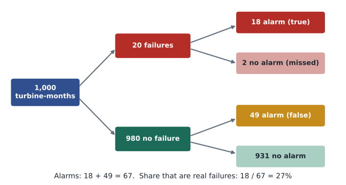
So the probability that an alarm signals a failing gearbox is 18 out of 67, about 27 percent. The test is useful: it raises the probability of failure from two percent to 27 percent, more than a thirteen-fold increase. But most alarms are still false, simply because healthy turbines vastly outnumber failing ones. This is the base-rate fallacy, and it appears wherever a rare condition is screened: fraud alerts on card transactions, security screening, medical tests, quality inspections and résumé filters.
Bayes' rule
The same calculation can be written as a formula named after Thomas Bayes, an eighteenth-century minister whose work was published after his death. It states that the probability of a hypothesis given the evidence equals the probability of the evidence given the hypothesis, multiplied by the prior probability of the hypothesis, divided by the overall probability of the evidence.
Substituting Owen's numbers gives 0.9 times 0.02 divided by the sum of 0.9 times 0.02 and 0.05 times 0.98, which is 0.018 divided by 0.067, or about 0.27. The formula and the natural-frequency tree give the same answer; the tree is easier to explain to a site manager, and the formula is easier to put into a spreadsheet or a program. Either way, Bayes' rule is simply a disciplined way of updating a belief when new evidence arrives.
# Probability of a real failure given an alarm, for different base rates
def p_fail_given_alarm(base_rate, sensitivity, false_alarm_rate):
    true_alarm = sensitivity * base_rate
    false_alarm = false_alarm_rate * (1 - base_rate)
    return true_alarm / (true_alarm + false_alarm)

for base in (0.005, 0.01, 0.02, 0.05, 0.10, 0.20):
    p = p_fail_given_alarm(base, 0.90, 0.05)
    print(f"Base rate {base:5.1%}  ->  chance an alarm is real {p:5.1%}")

# A second, independent alarm from a different sensor type raises it again
first = p_fail_given_alarm(0.02, 0.90, 0.05)
second = p_fail_given_alarm(first, 0.85, 0.08)
print(f"After one alarm {first:.1%}; after a second independent alarm {second:.1%}")Base rate 0.5% -> chance an alarm is real 8.3% Base rate 1.0% -> chance an alarm is real 15.4% Base rate 2.0% -> chance an alarm is real 26.9% Base rate 5.0% -> chance an alarm is real 48.6% Base rate 10.0% -> chance an alarm is real 66.7% Base rate 20.0% -> chance an alarm is real 81.8% After one alarm 26.9%; after a second independent alarm 79.6%
The output shows how strongly the answer depends on the base rate. On a turbine model where failures are rare, most alarms are false; on an older model where one turbine-month in five ends in failure, an alarm is right most of the time. It also shows the value of combining evidence. After one alarm, the probability becomes the new prior, and a second alarm from an independent check pushes it much higher. Owen's operations team settles on a two-step policy: an alarm triggers a remote review of the vibration data and an oil sample, which cost little, and only a second positive signal triggers a shutdown.
Thinking in expected costs
Probabilities alone do not tell a manager what to do; the costs of each kind of error matter too. A missed gearbox failure at Prairie Ridge can cost several hundred thousand dollars in repairs and weeks of lost output, while an unnecessary inspection costs perhaps fifteen thousand dollars. Even at a 27 percent chance of failure, shutting down might be worth it if the inspection is cheap relative to the damage it prevents. The expected cost of each action is the sum of each possible cost weighted by its probability. Lesson 11 develops this into a full decision analysis; for now the point is that a good decision combines the right probability with the right consequences.
| Action after one alarm | If gearbox failing (27%) | If gearbox healthy (73%) | Expected cost |
|---|---|---|---|
| Shut down and inspect | 15,000 inspection, failure avoided | 15,000 inspection | 15,000 |
| Remote review first | 2,000 review, then inspect: 17,000 (small risk of delay) | 2,000 review | about 6,100 |
| Ignore | 400,000 failure | 0 | about 108,000 |
The table is deliberately simplified, but it makes the logic visible. Ignoring the alarm has the highest expected cost because a failure is so expensive. The remote review is cheapest because it filters out most false alarms before the expensive step. The numbers that drive the answer, the cost of failure, the cost of inspection and the probability, can each be challenged and tested, which is far healthier than an argument about whether the system is reliable.
When independence fails
Many risk calculations multiply probabilities together on the assumption that events are independent. If each of three suppliers has a five percent chance of failing to deliver in a given month, the chance that all three fail at once would be 0.05 cubed, about one in eight thousand, if they were independent. But suppliers in the same region share the same weather, the same ports and the same labor market. A single storm or rail disruption can stop all three at once. The real probability of a joint failure may be many times higher than the independent calculation suggests.
The global financial crisis of 2007 to 2009 is the classic example: models of mortgage securities assumed that defaults in different regions were only weakly related, and house prices fell almost everywhere at once. Daniel recalls that Northfield's dual sourcing of steel coil gave little protection during the pandemic because both suppliers relied on the same mill. Dr. Zhou's advice is to look for common causes whenever a plan relies on several things not going wrong together, and to stress-test the plan with a scenario in which they all go wrong at the same time.
Probability words and calibration
Managers often express uncertainty in words rather than numbers: likely, probable, a real possibility, unlikely. Studies going back to work for the US intelligence community in the 1960s, and more recent surveys of thousands of people, show that readers interpret these words very differently. One person's likely is 60 percent and another's is 85 percent; a serious possibility can mean anything from 20 to 80 percent. Decisions made on the basis of such words can rest on a misunderstanding no one notices. Dr. Zhou asks the cohort to write down a number for each of five common phrases, and the spread of answers around the room makes the point at once.
The remedy is to use numbers, or agreed ranges, for important forecasts, and then to check whether they come true at the stated rate. A forecaster is well calibrated if, among all the events given a 70 percent probability, about 70 percent actually happen. Weather forecasters are known for good calibration because they receive rapid, clear feedback. Most managers are overconfident: when asked for a range they are 90 percent sure will contain a quantity, they produce ranges that capture the true value far less often. Keeping a simple record of forecasts and outcomes, and scoring them, is one of the cheapest ways for a team to improve its judgment.
The Brier score, devised by the meteorologist Glenn Brier in 1950, measures the accuracy of probability forecasts. For each forecast, subtract the outcome, coded one if the event happened and zero if it did not, from the stated probability, square the difference and average across forecasts. A perfect forecaster scores zero; someone who always says 50 percent scores 0.25. Leo starts tracking his sales team's probability estimates for deals closing each quarter and finds that deals rated 80 percent likely closed only about half the time, which explains his recurring revenue shortfalls.
Probability in everyday management
Dr. Zhou ends the session by asking each manager where conditional probability and base rates show up in their own work, and the answers fill a whiteboard. Grace's loss-prevention team relies on refund flags. Leo's sales team scores leads, and a lead score that is right most of the time for the large accounts it was built on may be poor for small retailers, where the base rate of buying is lower. Daniel's quality inspectors reject parts on the basis of automated vision checks, and he realizes he has never asked what share of rejected parts are actually defective; if it is low, the plant may be scrapping good parts and paying for it. Hana points to sepsis alerts in the hospital's electronic records, which nurses complain fire so often that they have begun to ignore them, a problem health systems describe as alert fatigue.
Alert fatigue is the human cost of the base-rate problem. When most alarms are false, people learn to dismiss them, and the rare true alarm is then missed. Owen's two-step policy addresses this directly: by sending only alarms that pass a cheap second check to the crew, he raises the share of shutdowns that find a real problem and protects the credibility of the system. The general lesson is that the value of any screening process depends on three numbers, not one: how common the problem is, how often the screen catches it, and how often it raises a false alarm. A vendor who quotes only the second is telling half the story, and a manager who asks for all three is in a position to judge whether the screen is worth its cost.
Worked problem
Screening for fraudulent refunds at Fairway
Fairway's loss-prevention team uses a rule that flags refund transactions as suspicious. About 0.5 percent of refunds are fraudulent. The rule flags 80 percent of fraudulent refunds and 3 percent of legitimate ones. The team wants to know what share of flagged refunds are fraudulent.
Show solution
- Imagine 100,000 refunds: 500 are fraudulent and 99,500 are legitimate.
- Flagged fraudulent refunds: 80 percent of 500 = 400.
- Flagged legitimate refunds: 3 percent of 99,500 = 2,985.
- Share of flags that are fraud: 400 divided by (400 + 2,985) = 400 / 3,385, about 11.8 percent.
Answer: Only about one flagged refund in eight or nine is fraudulent. Treating every flagged customer as a suspect would insult many honest customers; a better process uses the flag to prompt a light second check, such as a receipt look-up, and reserves confrontation for cases that fail it.
Common mistakes
MistakeA test that is 90 percent accurate means a positive result is 90 percent likely to be right.
InsteadThe chance a positive result is right depends heavily on the base rate; for rare conditions it can be low.
MistakeP(A given B) is the same as P(B given A).
InsteadThey point in different directions and can differ greatly; Bayes' rule connects them.
MistakeRisks can be multiplied together to find the chance they all occur.
InsteadOnly if they are independent; common causes make joint failures far more likely.
MistakeWords such as likely communicate uncertainty clearly.
InsteadPeople interpret probability words very differently; use numbers or agreed ranges.
Summary and key terms
- A conditional probability depends on what is known; P(A given B) and P(B given A) differ.
- Combine a base rate with test accuracy using natural frequencies or Bayes' rule.
- For rare conditions most alarms are false even with an accurate test; a second independent check helps.
- Choose actions by expected cost, combining probabilities with the cost of each error.
- Watch for common causes that break independence, and track and score probability forecasts.
- Conditional probability
- The probability of an event given that another event has occurred.
- Base rate
- How common a condition is before any test or signal is observed.
- Bayes' rule
- A formula for updating a probability in the light of new evidence.
- Independence
- Two events are independent when knowing one occurred does not change the probability of the other.
- Calibration
- The match between stated probabilities and how often events actually occur.
- Brier score
- The average squared difference between probability forecasts and outcomes; lower is better.
Practice problems
Work each problem on paper first, then reveal the answer to check.
A disease affects 1 in 1,000 people. A test detects 99 percent of cases and gives false positives for 2 percent of healthy people. What share of positive results are true cases?
Show answer
In 100,000 people: 100 cases, 99 detected; 99,900 healthy, 1,998 false positives. 99 divided by 2,097 is about 4.7 percent.
Three warehouses each have a 10 percent chance of flooding in a year. Why might the chance that all three flood be much higher than one in a thousand?
Show answer
They may share a river basin, a storm system or a drainage network, so their flood risks are correlated rather than independent.
A forecaster gives probabilities of 0.9, 0.6 and 0.2 for three events; the first two happen and the third does not. What is the Brier score?
Show answer
((0.9 - 1) squared + (0.6 - 1) squared + (0.2 - 0) squared) divided by 3 = (0.01 + 0.16 + 0.04) / 3 = 0.07.
Why is an alarm more trustworthy on an older turbine model with a higher failure rate?
Show answer
The base rate is higher, so a larger share of alarms come from real failures rather than healthy machines.
Lesson quiz · 5 questions
Score 60% or more to complete this lesson.
Create a free account to save your progress, take quizzes and earn a certificate.