
MBA-504 · Lesson 4 of 12 · 20 min
Sampling, surveys and confidence intervals
Leo Brandt's company, Kestrel Analytics, has about 2,600 retail customers. Last quarter the customer success team emailed a satisfaction survey to all of them and received 412 replies. Sixty-two percent said they were satisfied or very satisfied with the product, down from 68 percent in the previous survey. The board wants to know whether satisfaction has really fallen and, if so, whether to delay a planned price increase. Leo brings the results to Dr. Zhou's fourth session with two questions. How precise is a figure based on 412 replies? And can he trust the replies at all, given that more than four customers in five did not answer?
Dr. Zhou says the second question is more important than the first, and that managers usually ask them in the wrong order. Precision, the random wobble from sampling, can be calculated with a formula. Bias, the systematic error from who answers and how questions are asked, cannot be calculated and does not shrink with a larger sample. A huge biased sample gives a precise estimate of the wrong number.
Populations, samples and sampling frames
The population is the whole group a manager wants to learn about: all of Kestrel's customers, all the cars that come off a production line, all the patients who visit a clinic. A sample is the subset actually measured. The sampling frame is the list from which the sample is drawn, and it is often where problems begin. Kestrel's frame is its list of account administrators, the people who set up the software, but the people who use it every day are store and warehouse staff whose views may differ sharply. A survey of administrators cannot speak for users, however many administrators reply.
The gold standard is a random sample, in which every member of the population has a known chance of selection. Random selection does not guarantee a representative sample every time, but it ensures that the sample is not systematically skewed and allows the likely size of the sampling error to be calculated. Variants include stratified sampling, which draws separately from groups such as small, medium and large customers to ensure each is represented, and cluster sampling, which selects whole groups such as stores and then measures everyone in them, often to save travel or cost.
Sources of bias
Selection bias arises when the way the sample is chosen favors some members of the population. Online reviews come from people motivated to write them, often the very pleased and the very angry. Customers who stay long enough to be surveyed have already survived the churn that removed the unhappiest ones. Non-response bias arises when those who answer differ from those who do not. At Kestrel the response rate was 16 percent, and the customers who replied may be the more engaged ones, or those with a grievance. Response bias arises from how questions are asked: leading wording, a question that asks about two things at once, a scale that offers more positive than negative options, or the presence of an account manager when the customer answers.
The most famous illustration is the Literary Digest poll of the 1936 US presidential election. The magazine mailed about ten million ballots, drawn largely from lists of telephone owners, car owners and its own subscribers, and received more than two million replies, which predicted a comfortable win for Alf Landon. Franklin Roosevelt won in a landslide. The lists over-represented wealthier voters during the Depression, and those who chose to reply differed again. George Gallup, using a much smaller but more carefully selected sample, called the result correctly. Two million biased replies were worse than a few thousand chosen with care.
For Leo, the practical steps are clear. Compare respondents with the full customer list on things Kestrel already knows, such as company size, region, product tier and usage, and see whether any group is over- or under-represented. Weight the results to correct for known imbalances if needed. Follow up a small random sample of non-respondents by phone to see whether their answers differ. And keep the questionnaire identical between survey waves, because a change in wording can create an apparent change in satisfaction.
Sampling variation and the standard error
Even a perfectly random sample will not match the population exactly. If Kestrel drew many random samples of 412 customers, each would give a slightly different satisfaction rate, and these rates would cluster around the true population value. The spread of the estimates across repeated samples is called the standard error. For a proportion, it depends on the proportion itself and on the sample size.
With 62 percent satisfied in a sample of 412, the standard error is the square root of 0.62 times 0.38 divided by 412, which is about 0.024, or 2.4 percentage points. The crucial feature is the square root of n in the denominator. To halve the standard error, a survey needs four times as many responses. Going from 400 to 1,600 replies narrows the uncertainty by half; going from 1,600 to 6,400 narrows it by half again. Precision becomes expensive quickly, which is why national opinion polls rarely survey more than a few thousand people.
A remarkable fact, the central limit theorem, says that the distribution of a sample mean or proportion is approximately normal, the familiar bell curve, when the sample is reasonably large, whatever the shape of the underlying data. Grace's basket sizes are strongly skewed, but the average basket across many random samples of a few hundred transactions would follow a near-normal curve. This is what allows the same simple formulas to be used across so many business problems.
Confidence intervals
A confidence interval turns an estimate and its standard error into a range of plausible values for the population quantity. For a large sample, a 95 percent interval runs from about 1.96 standard errors below the estimate to 1.96 standard errors above. For Kestrel, that is 62 percent plus or minus 1.96 times 2.4 points, or roughly 57.3 to 66.7 percent. The half-width, here about 4.7 points, is the margin of error that news reports quote for opinion polls.
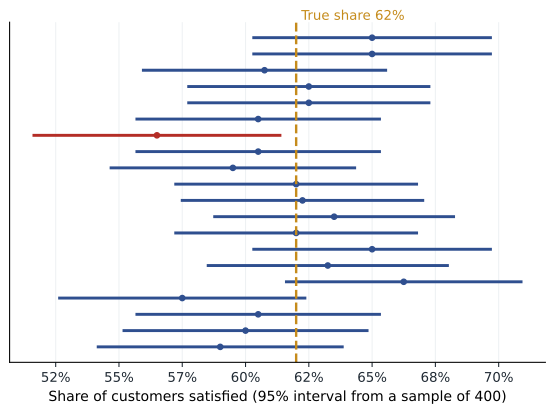
The meaning of the 95 percent is subtle. It describes the method, not the particular interval: if the survey were repeated many times and an interval calculated each time, about 95 percent of those intervals would contain the true value. Any single interval either contains it or does not. In practice, it is reasonable for a manager to treat the interval as the range of values consistent with the data, while remembering that it accounts only for random sampling error and not for bias.
# Confidence interval for a proportion, and a check of the 95 percent claim by simulation
import math, random
def ci_prop(successes, n, z=1.96):
    p = successes / n
    se = math.sqrt(p * (1 - p) / n)
    return p, p - z * se, p + z * se

p, lo, hi = ci_prop(255, 412)            # 255 of 412 respondents satisfied
print(f"Estimate {p:.1%}, 95% interval {lo:.1%} to {hi:.1%}, margin {hi - p:.1%}")

random.seed(1)
true_p, n, trials, hits = 0.62, 412, 2000, 0
for _ in range(trials):
    s = sum(random.random() < true_p for _ in range(n))
    _, a, b = ci_prop(s, n)
    hits += a <= true_p <= b
print(f"Share of {trials} simulated intervals containing the true value: {hits / trials:.1%}")Estimate 61.9%, 95% interval 57.2% to 66.6%, margin 4.7% Share of 2000 simulated intervals containing the true value: 95.1%
The simulation draws two thousand samples of 412 from a population in which exactly 62 percent are satisfied, builds an interval from each and counts how often the interval captures the truth. The answer is close to 95 percent, which is what the method promises when its assumptions hold.
Has satisfaction really fallen?
Leo's previous survey found 68 percent satisfied among 390 respondents. Its interval runs from about 63.4 to 72.6 percent. The two intervals overlap slightly, which suggests caution, although overlap of intervals is a conservative way to compare two estimates. A better approach, covered in the next lesson, is to construct an interval for the difference itself. The standard error of the difference between two independent proportions is the square root of the sum of their squared standard errors: about the square root of 0.024 squared plus 0.0236 squared, or 3.4 points. The observed difference of six points is about 1.8 standard errors, and a 95 percent interval for the change runs from roughly minus 12.6 to plus 0.6 points.
The data are therefore consistent with a fall of up to about twelve points but also with no change at all. Combined with the low response rate, Leo's honest message to the board is that the survey gives a warning sign, not proof. He recommends a short follow-up with a stratified random sample of 300 customers contacted by phone, which should reduce non-response bias, before deciding on the price increase. He also proposes tracking renewal rates and support tickets, which are measured for every customer and do not depend on who chooses to answer a survey.
Choosing a sample size
Before collecting data, a manager can decide how precise the result needs to be and work backwards to the sample size. Rearranging the margin of error formula, the sample needed for a margin of error m on a proportion is 1.96 squared times p times one minus p, divided by m squared. When there is no prior estimate, using p equal to 0.5 gives the most conservative answer, since p times one minus p is largest there.
For a margin of plus or minus three percentage points with p equal to 0.5, the formula gives 1.96 squared times 0.25 divided by 0.0009, about 1,067. For plus or minus five points it gives about 384. This is why so many polls survey about a thousand people. Note that the population size does not appear: a random sample of a thousand gives roughly the same precision for a city of a million as for a country of three hundred million, as long as the sample is a small fraction of the population. When the sample is a large fraction, as when Kestrel surveys several hundred of its 2,600 customers, a finite population correction narrows the interval somewhat, so the simple formula is slightly conservative.
| Desired margin of error | Sample needed (p = 0.5) | Sample needed (p = 0.2) |
|---|---|---|
| 10 points | 96 | 62 |
| 5 points | 384 | 246 |
| 3 points | 1,067 | 683 |
| 2 points | 2,401 | 1,537 |
| 1 point | 9,604 | 6,147 |
Intervals for averages
The same logic applies to averages. The standard error of a sample mean is the sample standard deviation divided by the square root of n, and a 95 percent interval is the mean plus or minus about two standard errors for large samples. For small samples the multiplier comes from the t distribution and is slightly larger, for example about 2.09 for 20 observations, to allow for the extra uncertainty in estimating the standard deviation. Hana uses this to estimate the average time nurses spend on discharge paperwork: a random sample of 36 discharges has a mean of 42 minutes and a standard deviation of 15 minutes, giving a standard error of 2.5 minutes and an interval of roughly 37 to 47 minutes.
Worked problem
Planning Fairway's shopper survey
Grace wants to estimate the share of Fairway shoppers who would use a new online ordering service, to within plus or minus four percentage points with 95 percent confidence. A pilot suggests about 30 percent interest. She expects only one in four people approached in store to agree to answer.
Show solution
- Apply the formula with p = 0.3: n = 1.96 squared times 0.3 times 0.7 divided by 0.04 squared.
- Calculate: 3.8416 times 0.21 = 0.8067; divided by 0.0016 gives about 504 completed surveys.
- Allow for the response rate: 504 divided by 0.25 means approaching about 2,000 shoppers.
- Reduce bias: spread interviews across stores, days and times so that weekday and weekend shoppers are both covered, and record refusals to compare with store traffic.
Answer: Grace plans for about 500 completed interviews, approaching about 2,000 shoppers across a schedule of stores and times. She also notes that stated interest usually overstates actual use, so she treats the result as an upper bound and plans a pilot in a few stores to measure real uptake.
Common mistakes
MistakeA larger sample removes bias.
InsteadSample size reduces random error only; a biased frame or low response can make a large sample misleading.
MistakeA 95 percent interval means there is a 95 percent chance the true value lies in this particular range.
InsteadStrictly, 95 percent of intervals built this way contain the truth; any one either does or does not.
MistakeThe sample must be a large share of the population to be useful.
InsteadPrecision depends mainly on the sample size, not the population size, for random samples.
MistakeA margin of error covers all sources of error.
InsteadIt covers only random sampling error, not wording, non-response or frame problems.
Summary and key terms
- Define the population and sampling frame, and draw a random or stratified sample where possible.
- Selection, non-response and response bias do not shrink with sample size.
- The standard error falls with the square root of n, so halving it needs four times the sample.
- A 95 percent interval is the estimate plus or minus about two standard errors.
- Plan sample sizes from the margin of error needed, then allow for the response rate.
- Population
- The whole group about which a conclusion is to be drawn.
- Sampling frame
- The list from which a sample is selected.
- Non-response bias
- Error arising when those who answer differ from those who do not.
- Standard error
- The typical size of the difference between a sample estimate and the population value across repeated samples.
- Confidence interval
- A range of plausible values for a population quantity, built from an estimate and its standard error.
- Margin of error
- The half-width of a confidence interval.
Practice problems
Work each problem on paper first, then reveal the answer to check.
A poll of 1,000 randomly selected voters finds 46 percent support for a policy. What is the 95 percent margin of error?
Show answer
1.96 times the square root of 0.46 times 0.54 divided by 1,000 = 1.96 times 0.0158, about 3.1 percentage points.
How many responses are needed for a margin of error of plus or minus 2 points on a proportion near 50 percent?
Show answer
1.96 squared times 0.25 divided by 0.0004, about 2,401.
A hotel leaves comment cards in rooms and 8 percent of guests return them. Why are the results unreliable as a measure of all guests' satisfaction?
Show answer
Guests who return cards choose to do so and are likely to differ from those who do not, often being more strongly positive or negative.
A sample of 25 invoices has a mean processing time of 6.2 days and a standard deviation of 2.5 days. Give an approximate 95 percent interval for the mean.
Show answer
Standard error = 2.5 / 5 = 0.5; with a t multiplier of about 2.06, the interval is 6.2 plus or minus 1.03, roughly 5.2 to 7.2 days.
Lesson quiz · 5 questions
Score 60% or more to complete this lesson.
Create a free account to save your progress, take quizzes and earn a certificate.