
MBA-504 · Lesson 10 of 12 · 20 min
Forecasting with time series
Every January, Lakeview Health's clinics are overwhelmed. Respiratory infections peak, the emergency department fills, and patients who cannot get a clinic appointment go to the hospital instead. Every summer the clinics are quiet and staff take leave. Hana Kowalski sets the clinic nursing schedule six months ahead, and last winter she under-staffed badly: visits ran about eight percent above the budget, which had been built by adding three percent to the previous year. Agency nurses filled the gaps at nearly twice the cost of staff nurses. Owen faces a similar problem at Prairie Ridge, where gas demand peaks in cold weather and wind output varies with the season. Dr. Zhou devotes the tenth session to forecasting, which she describes as the art of being usefully wrong.
What a time series contains
A time series is a sequence of measurements taken at regular intervals: monthly visits, weekly sales, daily electricity demand. Most business series can be thought of as a combination of four components. The trend is the long-run direction, such as Lakeview's gradual growth in visits as the population of its catchment area rises. Seasonality is a pattern that repeats over a fixed period, such as the winter peak in respiratory illness or the December peak in retail sales. Cycles are longer, irregular swings, often tied to the economy. And the remainder is the irregular noise that no model can predict.
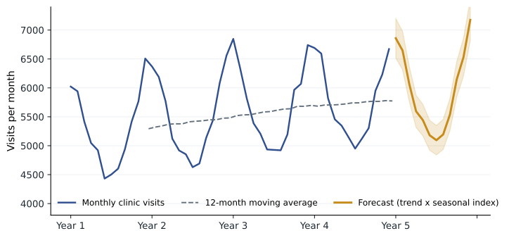
Hana's four years of monthly clinic visits show all of this clearly. Visits peak in December and January at around 6,500 to 6,800 a month and fall to about 4,500 to 5,000 in mid-summer. A twelve-month moving average, which averages each run of twelve consecutive months and so removes the seasonal pattern, rises steadily from about 5,300 to about 5,800 over the period. The first step in any forecast is to plot the series and identify these components; a forecast that ignores a strong seasonal pattern will be badly wrong at exactly the times that matter most.
Simple benchmarks
Before building anything sophisticated, a forecaster should establish simple benchmarks that any proposed method must beat. The naive forecast says that next period will equal this period. The seasonal naive forecast says that next January will equal last January, and so on for each month. The mean forecast uses the average of all past values. These sound crude, but they are surprisingly hard to beat for many series, and a method that cannot beat them on past data has no business being used.
The evidence from forecasting competitions supports this caution. The M competitions, organized by Spyros Makridakis and colleagues since 1982, have asked researchers and practitioners to forecast thousands of real time series, with results scored on data the forecasters had not seen. A recurring finding is that simple methods perform well relative to complex ones, and that combining the forecasts of several methods usually beats the individual methods. The M4 competition in 2018, with 100,000 series, found that most of the best performers were combinations, often mixing statistical and machine-learning methods. The M5 competition in 2020, using Walmart sales data, found that machine-learning methods could do well on large collections of related series, but the advantage came from careful engineering rather than from any single clever algorithm.
Moving averages and exponential smoothing
A moving average forecast predicts the next value as the average of the last k values. It smooths out noise, and a longer window smooths more but responds more slowly to real changes. Exponential smoothing refines this idea by giving the most recent observation the greatest weight and older observations geometrically decreasing weights. The forecast is updated each period by moving it part of the way toward the latest actual value.
The smoothing constant alpha controls how quickly the forecast reacts. With alpha near one, the forecast chases every movement; with alpha near zero, it barely moves. Simple exponential smoothing assumes no trend or seasonality, so on Hana's data it produces a flat forecast near recent levels and misses the winter peak entirely. Extensions add components: Holt's method adds a smoothed trend, and the Holt-Winters method adds smoothed seasonal factors as well. These methods, developed in the late 1950s and early 1960s for inventory control, remain among the most widely used forecasting tools in business, built into spreadsheets and planning software.
Seasonal indices and decomposition
A transparent way to handle seasonality is to compute a seasonal index for each month: the average value for that month divided by the overall average. An index of 1.17 for January means January visits typically run 17 percent above the average month; an index of 0.85 for July means July runs 15 percent below. Dividing each observation by its month's index gives a deseasonalized series, which shows the underlying trend more clearly. A trend line can be fitted to the deseasonalized data, projected forward and then multiplied by the seasonal index for each future month to produce the forecast.
Seasonal indices are also useful in their own right. Hana can use them to plan staffing for each month of the year in proportion to expected demand, and Grace's colleagues use them to judge whether a month's sales are good once the normal seasonal pattern has been taken into account. A report that December sales rose 30 percent over November says nothing if December always runs 35 percent above November; the deseasonalized change shows whether the business actually improved.
Measuring forecast accuracy
Forecast accuracy should be measured on data that were not used to build the forecast. A common approach is to hold back the most recent period, fit each method on the earlier data, forecast the held-back period and compare. Several measures are useful. The mean absolute error is the average size of the errors in the original units, such as visits. The mean absolute percentage error, or MAPE, expresses the average error as a percentage of the actual values, which allows comparison across series of different sizes, though it misbehaves when actual values are near zero. The root mean squared error penalizes large errors more heavily. And the bias, the average signed error, shows whether a method tends to forecast too high or too low; a biased forecast is a sign that something systematic has been missed.
# Backtest three forecasting methods on Lakeview's monthly clinic visits
import statistics
visits = [6022, 5941, 5417, 5046, 4922, 4432, 4504, 4604, 4940, 5419, 5767, 6507,
          6370, 6189, 5770, 5122, 4918, 4852, 4629, 4692, 5137, 5441, 6086, 6558,
          6847, 6348, 5815, 5387, 5209, 4935, 4928, 4921, 5195, 5966, 6070, 6740,
          6690, 6593, 5819, 5456, 5347, 5152, 4950, 5123, 5304, 5951, 6230, 6671]
train, test = visits[:36], visits[36:]          # fit on years 1 to 3, test on year 4

# 1. Seasonal naive: next January = last January, and so on
f_naive = train[-12:]

# 2. Simple exponential smoothing (no trend or season), alpha = 0.3
level = train[0]
for v in train[1:]:
    level = 0.3 * v + 0.7 * level
f_ses = [level] * 12

# 3. Seasonal index times linear trend
avg = statistics.mean(train)
index = [statistics.mean(train[m::12]) / avg for m in range(12)]
deseason = [v / index[i % 12] for i, v in enumerate(train)]
trend = statistics.linear_regression(range(36), deseason)
f_trend = [(trend.intercept + trend.slope * t) * index[t % 12] for t in range(36, 48)]

def scores(f):
    err = [a - b for a, b in zip(test, f)]
    mae = statistics.mean(abs(e) for e in err)
    mape = statistics.mean(abs(e) / a for e, a in zip(err, test))
    bias = statistics.mean(err)
    return mae, mape, bias
f_combo = [(a + b) / 2 for a, b in zip(f_naive, f_trend)]       # simple average of methods 1 and 3
for name, f in [('Seasonal naive', f_naive), ('Exponential smoothing', f_ses), ('Trend x seasonal index', f_trend), ('Average of 1 and 3', f_combo)]:
    mae, mape, bias = scores(f)
    print(f"{name:24s} MAE {mae:5.0f}   MAPE {mape:5.1%}   bias {bias:+5.0f}")
print("Seasonal index by month:", " ".join(f"{i:.2f}" for i in index))Seasonal naive MAE 117 MAPE 2.0% bias +77 Exponential smoothing MAE 574 MAPE 10.2% bias -178 Trend x seasonal index MAE 125 MAPE 2.1% bias -76 Average of 1 and 3 MAE 93 MAPE 1.6% bias +0 Seasonal index by month: 1.17 1.12 1.03 0.94 0.91 0.86 0.85 0.86 0.93 1.02 1.09 1.20
The backtest fits each method on the first three years and forecasts the fourth. Simple exponential smoothing, which ignores the seasonal pattern, has an average error of about 574 visits a month, or about ten percent. The seasonal naive forecast and the trend-times-seasonal-index forecast both do far better, at about two percent. The seasonal naive method tends to forecast slightly too low, because it ignores growth, while the trend method forecasts slightly too high. Their simple average cancels the biases and cuts the error to about 1.6 percent, a small-scale echo of the M competitions' finding that combinations usually win.
Forecast intervals and scenarios
A point forecast is almost certain to be wrong; the question is by how much. A forecast interval gives a range likely to contain the actual value, based on the size of past forecast errors. A useful rule of thumb is to look at the distribution of errors in the backtest and use, for example, the range covering 80 or 95 percent of them. Intervals should widen for forecasts further into the future, because errors accumulate. They should also be checked: if the 80 percent intervals from past forecasts contained the actual value only half the time, the intervals are too narrow, a common failing because forecasters tend to be overconfident.
Some uncertainties are better handled with scenarios than with intervals. An unusually severe respiratory season, a new clinic opening nearby, or a change in provincial or state funding could shift Hana's demand by more than any past pattern suggests. Planning for a base case, a high case and a low case, and deciding in advance what she would do in each, gives her a staffing plan that is robust rather than merely accurate on average. For Owen, the equivalent is to plan gas supply for a normal winter while holding contracts that can cover a cold-snap scenario.
Judgment and forecasting
Most organizations adjust statistical forecasts with human judgment, and the evidence on whether this helps is mixed. Studies of supply chain forecasting, including work by Robert Fildes and Paul Goodwin with several companies, found that large adjustments based on specific information, such as a planned promotion or a known store closure, often improved accuracy, while frequent small adjustments, especially upward ones driven by optimism, tended to make forecasts worse. The practical lessons are to adjust only when there is information the model does not have, to record the reason for each adjustment and to track whether adjustments improve accuracy over time.
Forecasts can also be distorted by incentives. Sales teams may lower forecasts so that targets are easier to beat; product managers may raise them to secure resources. Separating the forecast, an honest estimate of what will happen, from the target, what the organization wants to happen, and from the plan, what it will do about the difference, is one of the most useful disciplines a manager can introduce. Hana's budget had confused all three: the three percent growth figure was partly a forecast and partly a hope that visits would grow no faster than funding.
| Concept | Question it answers | Hana's example |
|---|---|---|
| Forecast | What do we expect to happen? | About 6,900 visits next January |
| Target | What do we want to happen? | Keep agency nurse cost below last year |
| Plan | What will we do? | Hire four seasonal nurses for November to March |
| Scenario | What if things differ sharply? | Severe season: open an extra evening clinic |
Forecasting demand, not sales
A final trap is that recorded sales or visits may not reflect true demand. When a store runs out of stock, sales stop even though shoppers still want the product; when a clinic is fully booked, patients who are turned away do not appear in the visit count. Forecasting from such censored data underestimates demand exactly when it is highest, and the forecast then justifies the same capacity that caused the shortfall. Hana adds a count of patients turned away or redirected to the emergency department to her data, so that next year's forecast reflects demand rather than the clinics' past capacity.
Worked problem
Building Hana's January staffing forecast
The trend fitted to Lakeview's deseasonalized visits implies an underlying level of about 5,900 visits a month next January, and January's seasonal index is 1.17. Backtest errors for January have ranged up to about 5 percent. Each nurse can handle about 360 visits a month.
Show solution
- Point forecast: 5,900 x 1.17, about 6,900 visits.
- Range: plus or minus 5 percent gives about 6,560 to 7,250 visits.
- Nurses needed: 6,900 / 360 is about 19.2 at the point forecast; 7,250 / 360 is about 20.1 at the top of the range.
- Plan: schedule 19 nurses plus a call-in pool able to cover one more, and set a trigger to open an extra evening clinic if weekly visits in early January run more than 10 percent above forecast.
Answer: Hana budgets for about 6,900 January visits and 19 nurses, with flexible capacity for a 20th. The plan links the forecast, its uncertainty and a pre-agreed response, rather than building a single number into the budget and hoping it is right.
Common mistakes
MistakeA sophisticated model will always beat a simple one.
InsteadSimple methods and combinations often forecast as well or better; test against benchmarks.
MistakeA forecast is a single number.
InsteadReport a range and plan for scenarios; point forecasts are almost always wrong.
MistakeForecast accuracy can be judged on the data used to build the model.
InsteadMeasure accuracy on held-out data that the model has not seen.
MistakePast sales measure past demand.
InsteadStockouts and capacity limits censor demand; record lost sales or turned-away customers.
Summary and key terms
- Time series combine trend, seasonality, cycles and noise; plot before modeling.
- Always compare methods with naive and seasonal naive benchmarks.
- Exponential smoothing weights recent data most; Holt-Winters adds trend and seasonality.
- Seasonal indices deseasonalize data and support trend-times-season forecasts.
- Measure accuracy with MAE, MAPE and bias on held-out data, combine methods, and keep forecasts separate from targets.
- Time series
- A sequence of observations recorded at regular time intervals.
- Seasonality
- A pattern that repeats over a fixed period such as a year or a week.
- Exponential smoothing
- A forecasting method that gives geometrically declining weights to older observations.
- Seasonal index
- The typical value for a season divided by the overall average.
- MAPE
- Mean absolute percentage error, the average absolute forecast error as a share of actual values.
- Forecast bias
- The tendency of forecasts to be systematically too high or too low.
Practice problems
Work each problem on paper first, then reveal the answer to check.
Monthly sales average 200 units overall and 260 units in December. What is December's seasonal index, and what does it mean?
Show answer
260 / 200 = 1.30: December sales typically run 30 percent above the average month.
The last forecast was 500 and the actual was 540. With alpha = 0.2, what is the next exponential smoothing forecast?
Show answer
0.2 x 540 + 0.8 x 500 = 108 + 400 = 508.
Three months have actual values of 100, 120 and 80 and forecasts of 110, 114 and 90. Compute the MAPE.
Show answer
Absolute percentage errors are 10 percent, 5 percent and 12.5 percent; the MAPE is about 9.2 percent.
A planner's forecasts have been too high in 10 of the last 12 months. What does this suggest, and what should be done?
Show answer
The forecasts are biased upward, perhaps from optimism or incentives; review the method and any judgmental adjustments and track bias going forward.
Lesson quiz · 5 questions
Score 60% or more to complete this lesson.
Create a free account to save your progress, take quizzes and earn a certificate.