
MBA-504 · Lesson 7 of 12 · 20 min
Correlation, causation and confounding
Daniel Osei has been asked by Northfield's general manager to cut overtime. The argument seems compelling: a chart from the quality team shows that the defect rate on overtime shifts is 4.8 percent, against 2.8 percent on regular shifts, and the general manager concludes that tired workers make more mistakes. Reducing overtime would save money and improve quality at the same time. Daniel is skeptical. Overtime at Northfield is concentrated on large, complex welded assemblies for a truck manufacturer, and those jobs have always had higher defect rates. Dr. Zhou tells him he has just described the most important trap in business analysis.
Measuring association: the correlation coefficient
When two numerical variables tend to move together, they are said to be correlated. The Pearson correlation coefficient, usually written r, measures the strength and direction of a straight-line relationship on a scale from minus one to plus one. A value near plus one means that high values of one variable go with high values of the other; near minus one, high values of one go with low values of the other; near zero, there is no straight-line relationship. It is calculated from the standardized values of the two variables, so it does not depend on the units of measurement.
Correlation has well-known limitations. It measures only straight-line association, so a strong curved relationship, such as the way sales respond to advertising with diminishing returns, can produce a modest r. A single outlier can create or destroy a correlation. Correlations computed on averages for groups, such as stores or regions, are usually much stronger than those for the individuals within them. And a correlation coefficient says nothing about the size of the effect: a correlation of 0.3 between training hours and productivity could mean a large or a trivial gain per hour. Always plot the data before trusting r.
Three reasons two things move together
When two variables are correlated, there are three broad explanations apart from chance. The first is that one causes the other, as the general manager assumes: overtime causes fatigue, which causes defects. The second is reverse causation: the outcome drives the supposed cause. Perhaps defects cause overtime, because rework on defective parts must be done after hours. The third is confounding: a third factor drives both. At Northfield, complex jobs both require more overtime, because they take longer and have tight deadlines, and produce more defects, because they involve more welds and tighter tolerances.
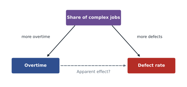
Diagrams like this, which researchers call causal graphs, are a simple but powerful tool for managers. Draw the variables, add arrows for the causal links you believe exist, and look for paths that connect the supposed cause and the effect through a third variable. Any such path through a common cause is a source of confounding that must be dealt with before the association can be read as an effect. The computer scientist Judea Pearl, who formalized these methods, argues that causal questions cannot be answered from data alone without some assumptions about how the world works; the diagram makes those assumptions explicit and open to challenge.
Simpson's paradox
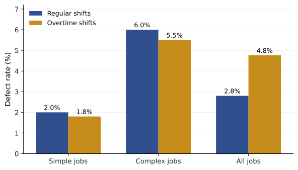
Daniel splits the defect data by job type, and the picture reverses. On simple jobs, overtime shifts have a defect rate of 1.8 percent against 2.0 percent on regular shifts. On complex jobs, overtime shifts run at 5.5 percent against 6.0 percent on regular shifts. Within each type of job, overtime shifts are slightly better, not worse. The overall comparison makes overtime look bad only because most overtime shifts work on complex jobs, while most regular shifts work on simple ones.
| Job type | Regular shifts: units, defects, rate | Overtime shifts: units, defects, rate |
|---|---|---|
| Simple | 8,000, 160, 2.0% | 2,000, 36, 1.8% |
| Complex | 2,000, 120, 6.0% | 8,000, 440, 5.5% |
| All jobs | 10,000, 280, 2.8% | 10,000, 476, 4.8% |
This reversal is known as Simpson's paradox, after the statistician Edward Simpson, who described it in 1951. A famous real example came from graduate admissions at the University of California, Berkeley, in 1973. Overall, men were admitted at a noticeably higher rate than women, which looked like discrimination. When the statisticians Peter Bickel, Eugene Hammel and J. W. O'Connell examined admissions department by department, they found that most departments admitted women at similar or higher rates. Women had applied disproportionately to departments with low admission rates for everyone. The paradox is not a statistical curiosity; it arises whenever the mix of groups differs between the things being compared.
# Simpson's paradox in Northfield's defect data (units and defective units)
data = {                       # job type: (regular units, regular defects, overtime units, overtime defects)
    'Simple':  (8000, 160, 2000, 36),
    'Complex': (2000, 120, 8000, 440),
}
tot = [0, 0, 0, 0]
for job, (ru, rd, ou, od) in data.items():
    print(f"{job:8s} regular {rd / ru:5.1%}   overtime {od / ou:5.1%}")
    tot = [a + b for a, b in zip(tot, (ru, rd, ou, od))]
print(f"{'All':8s} regular {tot[1] / tot[0]:5.1%}   overtime {tot[3] / tot[2]:5.1%}")

# Standardize: apply each shift type's rates to the same 50/50 job mix
mix = {'Simple': 0.5, 'Complex': 0.5}
reg = sum(mix[j] * d[1] / d[0] for j, d in data.items())
ot = sum(mix[j] * d[3] / d[2] for j, d in data.items())
print(f"Same job mix: regular {reg:.2%}, overtime {ot:.2%}")Simple regular 2.0% overtime 1.8% Complex regular 6.0% overtime 5.5% All regular 2.8% overtime 4.8% Same job mix: regular 4.00%, overtime 3.65%
Standardizing to a common job mix gives a fair comparison: with the same mix of work, overtime shifts would have a slightly lower defect rate. This does not prove that overtime is harmless; there may be other differences between shifts, and very long hours may still cause problems that this aggregate data cannot show. But it removes the main argument for the general manager's conclusion and redirects attention to the real driver of defects, which is the complex truck assemblies.
Selection and survivorship
A different trap arises when the data include only cases that passed through some filter. During the Second World War, the statistician Abraham Wald worked with the US military on where to add armor to bombers. The planes that returned from missions showed bullet holes concentrated on the wings and fuselage. The intuitive response was to reinforce those areas. Wald's insight, as the story is usually told, was that the data came only from planes that survived; planes hit in the engines did not come back. The armor belonged where the returning planes had no holes.
Survivorship bias is common in business. Studies of successful companies identify habits that unsuccessful companies may have shared. Analyses of current customers miss those who left. Fund managers' track records omit funds that closed after poor results. Hana notices it in Lakeview's data: patients who completed a rehabilitation program had much better outcomes than those who did not, but patients who dropped out were often those whose health deteriorated, so completion partly reflects health rather than causing it. Whenever data come from a filtered group, ask what the filter removed.
Getting closer to causes without an experiment
Randomized experiments are the most reliable way to establish cause and effect, but they are not always possible. A company cannot randomly assign which plants unionize, which managers are promoted or which regions suffer a recession. Several approaches can help, each with assumptions that should be stated plainly.
The first is to control for confounders, either by comparing like with like, as Daniel did by splitting by job type, or by including the confounders in a regression model, covered in the next two lessons. This works only for confounders that are measured; it cannot fix bias from those that are not. The second is difference-in-differences, introduced in lesson 6: compare the change over time in a group affected by some event with the change in a similar unaffected group. The key assumption is that the two groups would have followed parallel paths without the event. The third is to look for natural experiments, in which chance or an arbitrary rule assigns treatment. Regression discontinuity designs exploit cut-offs: customers just above and just below a loyalty-tier threshold, or students just above and below an admission score, are very similar except for the treatment.
| Approach | Key assumption | Business example |
|---|---|---|
| Randomized experiment | Random assignment carried out correctly | A/B test of a checkout page |
| Control for confounders | All important confounders are measured | Comparing defect rates within job type |
| Difference-in-differences | Groups would have moved in parallel | Stores with and without a new layout, before and after |
| Regression discontinuity | Units just either side of a cut-off are comparable | Customers just above and below a loyalty threshold |
| Natural experiment | Assignment is as good as random | A lottery for limited training places |
Questions to ask of a causal claim
Dr. Zhou suggests a short checklist for any claim that one thing causes another. Is there a plausible mechanism? Does the cause come before the effect in time? Is the association strong, and does it grow with the dose, such as more hours of overtime bringing more defects? Has it been found consistently in different settings and by different methods? Have the obvious confounders been considered and measured? And could the direction run the other way? These questions echo criteria proposed by the epidemiologist Austin Bradford Hill in 1965 for judging whether an association, such as that between smoking and lung cancer, reflects causation. No single criterion is decisive, but a claim that fails several deserves skepticism.
Daniel takes the analysis back to the general manager. Overtime is not the cause of Northfield's quality problem; complex jobs are. Cutting overtime would delay the truck orders without improving quality. Instead, Daniel proposes a small experiment: for six weeks, half of the complex-job teams, chosen at random, will be capped at ten hours per shift while the others continue as before. This will test the fatigue hypothesis directly, and the quality engineers will meanwhile study which weld types account for most defects on the complex assemblies.
Causal thinking in everyday decisions
The cohort quickly finds examples of the same trap in their own organizations. Grace's marketing colleagues report that customers who receive the most promotional emails spend the most, and want to send more emails to everyone. But the email system targets customers who have bought recently, so heavy spenders receive more emails because they spend, not the other way around. Leo's sales data show that customers assigned a dedicated success manager churn less, yet success managers are assigned to the largest and most committed accounts. Hana's clinics see that patients who use the online portal have fewer emergency visits, but portal users tend to be younger and healthier. Each comparison mixes the effect of the intervention with the characteristics of those who received it.
In each case the remedy follows the same pattern. Draw the causal diagram and identify why some units received the treatment. If treatment was targeted on the basis of something that also predicts the outcome, the raw comparison is confounded. Compare like with like on the targeting variables, look for a natural experiment, or, best of all, randomize who receives the treatment for a period. Grace's team runs a holdout test in which a random ten percent of customers receive no promotional emails for a quarter. The difference in spending between the holdout and everyone else measures what the emails actually achieve, and it turns out to be positive but much smaller than the raw comparison suggested, which leads the team to cut email frequency for customers who show no response.
Worked problem
Testing a claim about Kestrel's training webinars
Kestrel's customer success team reports that customers who attended an onboarding webinar renewed at 91 percent, compared with 74 percent for those who did not. They want to make the webinar mandatory, claiming it would lift renewals by 17 points.
Show solution
- List alternative explanations: customers who attend may already be more engaged, have larger teams or have a dedicated administrator, all of which predict renewal (confounding).
- Check for reverse direction: customers who already planned to expand might attend to learn new features.
- Compare like with like: within customer size bands and usage levels, the renewal gap shrinks to about 6 points.
- Propose a test: randomly invite half of new customers to a personal webinar booking and compare renewal between the invited and not-invited groups.
Answer: Leo concludes that the webinar may help but that the 17-point gap is mostly selection. An experiment based on random invitations will measure the true effect of encouraging attendance, which is the decision Kestrel actually faces.
Common mistakes
MistakeA strong correlation shows that one variable causes the other.
InsteadConfounding, reverse causation and chance can all produce correlation.
MistakeIf a comparison holds overall, it holds within every group.
InsteadSimpson's paradox shows the direction can reverse when group mix differs.
MistakeData on current customers or survivors tell the full story.
InsteadSurvivorship bias hides those who left or failed; ask what the filter removed.
MistakeControlling for variables in a model removes all confounding.
InsteadOnly measured confounders are controlled; unmeasured ones remain.
Summary and key terms
- The correlation coefficient measures straight-line association from minus one to plus one; plot the data first.
- Correlation can arise from causation, reverse causation, confounding or chance.
- Draw a causal diagram to identify confounders and make assumptions explicit.
- Simpson's paradox and survivorship bias show how group mix and filtering mislead.
- Without experiments, use controls, difference-in-differences or natural experiments, stating their assumptions.
- Correlation coefficient
- A measure of the strength and direction of a straight-line relationship between two variables.
- Confounder
- A variable that influences both a supposed cause and its outcome.
- Reverse causation
- When the outcome influences the supposed cause.
- Simpson's paradox
- A reversal of an association when data are split into groups.
- Survivorship bias
- Error from analyzing only cases that passed through a selection process.
- Natural experiment
- A situation in which chance or an arbitrary rule assigns treatment, allowing causal comparison.
Practice problems
Work each problem on paper first, then reveal the answer to check.
Cities with more police officers have more crime. Give two explanations other than police causing crime.
Show answer
Reverse causation: cities with more crime hire more police. Confounding: larger, denser cities have both more crime and more police.
Hospital A has a higher overall death rate than Hospital B, yet a lower death rate for both low-risk and high-risk patients. How is this possible?
Show answer
Hospital A treats a much larger share of high-risk patients, so its overall rate is pulled up by its case mix: an instance of Simpson's paradox.
A study of successful start-ups finds most founders dropped out of university. Why is this weak evidence that dropping out helps?
Show answer
It ignores the many dropouts whose start-ups failed; looking only at successes creates survivorship bias.
What is the key assumption of a difference-in-differences comparison?
Show answer
That the treated and comparison groups would have followed parallel trends in the absence of the treatment.
Lesson quiz · 5 questions
Score 60% or more to complete this lesson.
Create a free account to save your progress, take quizzes and earn a certificate.