
MBA-504 · Lesson 11 of 12 · 21 min
Decision analysis: decision trees, expected value and the value of information
Prairie Ridge Energy owns a gas processing plant in a region where several producers are drilling new wells. If drilling goes well, the plant will need far more capacity within three years; if it disappoints, existing capacity will be enough. Owen Tremblay has been asked to recommend whether to build a large expansion, a small one or none at all. The engineering team favors the large expansion, which would capture the most business if volumes grow. The finance committee worries that an oversized plant would lose money for years if they do not. A consultancy has offered to carry out a geological and market study for 1.5 million dollars, and Owen must also decide whether that study is worth buying. Dr. Zhou's eleventh session brings together probability, data and judgment in a single framework: decision analysis.
Structuring a decision under uncertainty
A decision problem has three elements: the alternatives the decision-maker controls, the uncertain events that will affect the outcome, and the payoffs that result from each combination. Writing them down is often the most valuable step, because it forces a team to agree on what is being decided, what could happen and how outcomes will be valued. Owen's team agrees that demand will be either high or low, that the planning team's best estimate of high demand is 40 percent, and that payoffs will be measured as net present value in millions of dollars, using the company's cost of capital, a concept the cohort will study in finance.
| Alternative | High demand (p = 0.4) | Low demand (p = 0.6) | Expected value |
|---|---|---|---|
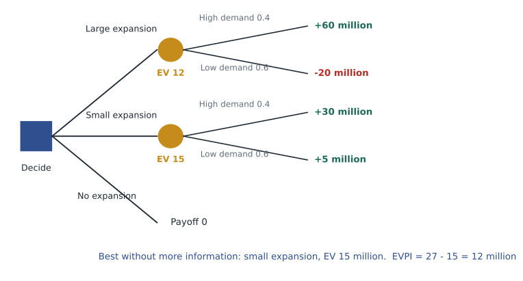
| Large expansion | +60 | -20 | 0.4 x 60 + 0.6 x (-20) = 12 |
| Small expansion | +30 | +5 | 0.4 x 30 + 0.6 x 5 = 15 |
| No expansion | 0 | 0 | 0 |
Decision criteria
Several rules can be used to choose among alternatives, and they reflect different attitudes to uncertainty. The optimist's rule, maximax, picks the alternative with the best possible outcome: the large expansion, with its 60 million upside. The pessimist's rule, maximin, picks the alternative whose worst outcome is least bad: the small expansion, whose worst case is still a gain of 5 million. The minimax regret rule considers how much one might regret each choice once the outcome is known. If demand is high, choosing small leaves 30 million on the table; if demand is low, choosing large costs 25 million relative to small. The large expansion has the smaller maximum regret, 25 against 30.
These rules ignore probabilities, which is their weakness when reasonable probability estimates exist. The expected value rule weights each payoff by its probability and picks the alternative with the highest average. On Owen's numbers, the small expansion has the highest expected value, 15 million, against 12 million for the large expansion. Expected value is the natural criterion for a firm that makes many decisions of similar size, because over many decisions the average outcome is what accumulates. For a decision large enough to threaten the firm, risk attitude matters too, as discussed below.
Decision trees
A decision tree draws the problem as a sequence of choices and chance events. Squares represent decisions, circles represent chance events, and the branches end in payoffs. The tree is solved by rolling back from right to left: at each chance node, compute the expected value of its branches; at each decision node, choose the branch with the highest value. Trees become indispensable when decisions unfold in stages, for example when the firm can first buy information, then decide, then learn the outcome.
The expected value of perfect information
Before paying for the study, Owen asks how much any information could possibly be worth. Suppose a perfectly reliable oracle could reveal in advance whether demand will be high or low. If it said high, Owen would build large and earn 60 million; if low, he would build small and earn 5 million. Since the oracle will say high 40 percent of the time, the expected value with perfect information is 0.4 times 60 plus 0.6 times 5, or 27 million. The expected value of perfect information, EVPI, is the difference between this and the best he can do without information: 27 minus 15, or 12 million. No study, however good, can be worth more than 12 million to this decision.
EVPI is a powerful screening tool. Many organizations spend heavily on research for decisions where the value of even perfect information is small, because the best choice is the same whatever happens or because the stakes are modest. Conversely, they sometimes skimp on information for decisions where the EVPI is large. Asking what perfect information would be worth takes minutes and frames the discussion about whether to commission research.
The expected value of sample information
Real studies are imperfect. The consultancy's track record suggests that when demand turns out high, its study gives a positive report 80 percent of the time; when demand turns out low, it gives a positive report 20 percent of the time. To value the study, Owen must work out what he would do after each possible report and how likely each report is, using Bayes' rule from lesson 3.
The probability of a positive report is 0.8 times 0.4 plus 0.2 times 0.6, or 0.44. After a positive report, the probability of high demand rises to 0.32 divided by 0.44, about 0.73; after a negative report it falls to 0.08 divided by 0.56, about 0.14. With a positive report the large expansion has an expected value of about 38.2 million and is the best choice; with a negative report the small expansion is best, at about 8.6 million. Weighting by the probability of each report, the expected value with the study is 0.44 times 38.2 plus 0.56 times 8.6, about 21.6 million. The expected value of sample information is 21.6 minus 15, or 6.6 million. Since the study costs 1.5 million, it is well worth buying.
# Rolling back Owen's decision tree, with perfect and sample information
p_high = 0.4
payoff = {'Large': (60, -20), 'Small': (30, 5), 'None': (0, 0)}     # million dollars: (high, low)

def best(p):
    ev = {k: p * h + (1 - p) * l for k, (h, l) in payoff.items()}
    choice = max(ev, key=ev.get)
    return choice, ev[choice], ev

choice, ev_now, all_ev = best(p_high)
print("Expected values now:", {k: round(v, 1) for k, v in all_ev.items()}, "-> choose", choice)

ev_perfect = p_high * max(h for h, _ in payoff.values()) + (1 - p_high) * max(l for _, l in payoff.values())
print(f"EV with perfect information {ev_perfect:.1f}; EVPI {ev_perfect - ev_now:.1f}")

# Market study: positive result with prob 0.8 if demand is high, 0.2 if low
pos_if_high, pos_if_low = 0.8, 0.2
p_pos = pos_if_high * p_high + pos_if_low * (1 - p_high)
p_high_pos = pos_if_high * p_high / p_pos
p_high_neg = (1 - pos_if_high) * p_high / (1 - p_pos)
c_p, ev_p, _ = best(p_high_pos)
c_n, ev_n, _ = best(p_high_neg)
ev_study = p_pos * ev_p + (1 - p_pos) * ev_n
print(f"P(positive) {p_pos:.2f}; P(high | positive) {p_high_pos:.3f}; P(high | negative) {p_high_neg:.3f}")
print(f"If positive choose {c_p} (EV {ev_p:.1f}); if negative choose {c_n} (EV {ev_n:.1f})")
print(f"EV with study {ev_study:.1f}; EVSI {ev_study - ev_now:.1f}")

# Break-even probability between large and small expansion
(hl, ll), (hs, ls) = payoff['Large'], payoff['Small']
print(f"Large beats small when P(high) exceeds {(ls - ll) / ((hl - ll) - (hs - ls)):.3f}")Expected values now: {'Large': 12.0, 'Small': 15.0, 'None': 0.0} -> choose Small
EV with perfect information 27.0; EVPI 12.0
P(positive) 0.44; P(high | positive) 0.727; P(high | negative) 0.143
If positive choose Large (EV 38.2); if negative choose Small (EV 8.6)
EV with study 21.6; EVSI 6.6
Large beats small when P(high) exceeds 0.455The calculation also shows why the study has value: it can change the decision. Without information, Owen would build small. With a positive report, he would switch to large. Information is valuable only when some possible result would lead to a different action; a study whose every possible result would leave the decision unchanged is worth nothing for that decision, however interesting its findings.
Sensitivity analysis
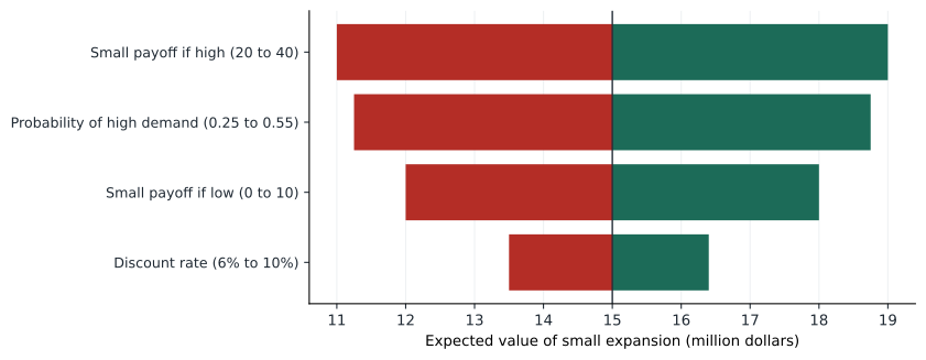
Every input to a decision analysis is an estimate, and some matter more than others. Sensitivity analysis varies each input across a plausible range and records how the result changes. The break-even probability is a good starting point: the large expansion beats the small one when the probability of high demand exceeds about 0.455. Owen's estimate of 0.4 is not far below this, so the choice is close and the study, which sharpens the probability, is especially valuable.
A tornado diagram displays one-way sensitivity analysis for several inputs at once. Each bar shows how far the expected value of the preferred alternative moves when one input swings from its low to its high value with the others held fixed, and the bars are sorted with the widest at the top, giving the funnel shape that names the chart. The inputs with the widest bars are where better estimates are most valuable, and where management attention should go.
Simulation
Decision trees with a few branches cannot capture uncertainty that is continuous, such as a range of possible volumes, prices and costs. Monte Carlo simulation, named after the casino, handles this by drawing random values for each uncertain input from a probability distribution, computing the outcome, and repeating thousands of times. The result is a distribution of outcomes rather than a single expected value, which shows the range of possibilities and the probability of a loss.
# Monte Carlo: how often does the large expansion beat the small one?
import random, statistics
random.seed(11)
runs, large_wins, diff = 20000, 0, []
for _ in range(runs):
    p = random.uniform(0.25, 0.55)                       # uncertain chance of high demand
    high = random.random() < p                            # the demand that actually occurs
    large = random.triangular(40, 75, 60) if high else random.triangular(-35, -10, -20)
    small = random.triangular(20, 40, 30) if high else random.triangular(0, 10, 5)
    large_wins += large > small
    diff.append(large - small)
print(f"Large expansion ends up better in {large_wins / runs:.0%} of simulated futures")
print(f"Average advantage of small over large: {-statistics.mean(diff):.1f} million")
q = statistics.quantiles(diff, n=20)
print(f"Middle 90% of (large minus small): {q[0]:.1f} to {q[-1]:.1f} million")Large expansion ends up better in 40% of simulated futures Average advantage of small over large: 4.9 million Middle 90% of (large minus small): -35.0 to 37.8 million
The simulation treats both the probability of high demand and each payoff as uncertain. In about 40 percent of simulated futures the large expansion turns out better, but the small expansion is better on average by about 5 million, and the difference between them ranges widely. The distribution makes plain what the single expected value hides: the choice is a gamble either way, and the size of the downside under the large expansion is substantial.
Risk attitude and staged decisions
Expected value treats a certain 15 million as equivalent to a gamble with the same average. For decisions small relative to the firm, that is reasonable. For a decision that could weaken the balance sheet or cost managers their jobs, many decision-makers prefer less risk and will accept a lower expected value to get it. Decision analysts capture this with a utility function, which converts payoffs into a measure of satisfaction that rises less steeply for gains than losses hurt. The certainty equivalent of a gamble is the sure amount the decision-maker would accept in its place; for a risk-averse decision-maker, it is less than the expected value. Prairie Ridge's board, with a loan covenant that would be strained by a 20 million loss, behaves in a risk-averse way, which strengthens the case for the small expansion or for buying information.
Often the best response to uncertainty is to avoid committing everything at once. Owen's engineers point out that the small expansion can be designed so that a second phase could be added later, at somewhat higher total cost than building large at the start. This option to expand has value: Prairie Ridge would build small now and add the second phase only if drilling results are strong. Such staged decisions, which finance calls real options, often beat both the cautious and the bold alternatives, because they let the firm learn before making the irreversible part of the investment. The cohort's finance course will value these options more formally.
Worked problem
Valuing a pilot for Kestrel's new product
Leo is considering launching a pricing-optimization module. A full launch would earn a net present value of 8 million dollars if the market is receptive (probability 0.5) and lose 4 million if not. A three-month pilot with five customers would cost 0.5 million. The pilot is positive 90 percent of the time when the market is receptive and 30 percent of the time when it is not.
Show solution
- Without information: EV of launch = 0.5 x 8 + 0.5 x (-4) = 2 million, better than not launching (0), so launch.
- EVPI: with perfect information, launch only if receptive: 0.5 x 8 = 4 million; EVPI = 4 - 2 = 2 million.
- Pilot results: P(positive) = 0.9 x 0.5 + 0.3 x 0.5 = 0.6. P(receptive | positive) = 0.45 / 0.6 = 0.75; P(receptive | negative) = 0.05 / 0.4 = 0.125.
- Decisions after the pilot: if positive, launch EV = 0.75 x 8 + 0.25 x (-4) = 5; if negative, launch EV = 0.125 x 8 + 0.875 x (-4) = -2.5, so do not launch (0). EV with pilot = 0.6 x 5 + 0.4 x 0 = 3 million.
Answer: The pilot's expected value of sample information is 3 minus 2, or 1 million, which exceeds its 0.5 million cost. Leo should run the pilot and launch only if it is positive.
Common mistakes
MistakeDecision analysis requires precise probabilities.
InsteadRough estimates plus sensitivity analysis reveal whether the choice depends on them.
MistakeInformation is always worth having.
InsteadInformation is valuable only if it could change the decision; EVPI caps its value.
MistakeA good decision is one that turns out well.
InsteadJudge decisions by the quality of reasoning given what was known; good decisions can have bad outcomes.
MistakeThe choice is between committing fully and doing nothing.
InsteadStaged decisions and options often let the firm learn before committing.
Summary and key terms
- Structure decisions as alternatives, uncertain events and payoffs, and roll back decision trees from right to left.
- Maximax, maximin and minimax regret ignore probabilities; expected value uses them.
- EVPI caps what any information is worth; EVSI uses Bayes' rule to value an imperfect study.
- Sensitivity analysis, break-even probabilities, tornado diagrams and simulation show which inputs matter.
- Account for risk attitude and look for staged decisions that preserve options.
- Payoff table
- A table of outcomes for each combination of alternative and uncertain state.
- Expected value
- The probability-weighted average of possible payoffs.
- Decision tree
- A diagram of decisions, chance events and payoffs, solved by rolling back.
- EVPI
- The expected value of perfect information: the most any information could be worth.
- EVSI
- The expected value of sample information from an imperfect study.
- Certainty equivalent
- The sure amount a decision-maker considers equal to a risky gamble.
Practice problems
Work each problem on paper first, then reveal the answer to check.
An investment pays 50 with probability 0.3 and minus 10 with probability 0.7. What is its expected value?
Show answer
0.3 x 50 + 0.7 x (-10) = 15 - 7 = 8.
Using Owen's payoffs, what is the expected value of the large expansion if the probability of high demand is 0.5?
Show answer
0.5 x 60 + 0.5 x (-20) = 20 million, which now beats the small expansion at 0.5 x 30 + 0.5 x 5 = 17.5 million.
A firm's best alternative has an EV of 10 million; with perfect information its EV would be 13 million. A consultant offers a study for 4 million. Should it consider buying?
Show answer
No: the EVPI is 3 million, so no study can be worth 4 million to this decision.
Why might a firm choose an alternative with a lower expected value?
Show answer
If it is risk-averse and the higher-EV alternative carries a downside large enough to threaten the firm, the lower-risk alternative may have a higher certainty equivalent.
Lesson quiz · 5 questions
Score 60% or more to complete this lesson.
Create a free account to save your progress, take quizzes and earn a certificate.