
MBA-504 · Lesson 5 of 12 · 20 min
Hypothesis testing and A/B experiments
Kestrel Analytics offers a free thirty-day trial, and the share of website visitors who start one is a number Leo watches closely. The marketing team has redesigned the trial sign-up page with a shorter form and a customer quote, and instead of simply switching to the new page they ran an experiment. For two weeks, each visitor was randomly shown either the current page or the new one. Of 4,000 visitors who saw the current page, 400 started a trial, a rate of 10.0 percent. Of 4,000 who saw the new page, 456 started a trial, a rate of 11.4 percent. The marketing head wants to roll out the new page at once. Leo wants to know whether a 1.4-point difference could simply be chance. This is the question hypothesis testing was designed to answer.
Why randomized experiments are special
Most business data are observational: they record what happened, without anyone controlling who received what. Observational comparisons are vulnerable to confounding, in which some third factor drives both the treatment and the outcome. If Kestrel had shown the new page only to visitors arriving from a partner's website, any difference might reflect those visitors rather than the page. Random assignment solves this problem. Because a coin flip decides who sees which version, the two groups are alike on average in every respect, measured or not, except for the page itself. Any systematic difference in outcomes can then be attributed to the change, with chance as the only alternative explanation.
This logic, developed by the statistician Ronald Fisher for agricultural trials in the 1920s and 1930s, underpins clinical trials of new drugs and, increasingly, management. Large online firms run many thousands of controlled experiments a year on their websites and apps, and experimentation platforms have made the method available to much smaller companies. Ronny Kohavi and colleagues, who led experimentation at Microsoft and other firms, report that most ideas tested in this way fail to improve the metric they were designed to move, which is a humbling reminder of how often intuition is wrong.
The logic of a hypothesis test
A hypothesis test starts by assuming the dull explanation: the change made no difference. This is the null hypothesis. The alternative hypothesis is that it did make a difference. The test then asks how surprising the observed data would be if the null hypothesis were true. If the data would be very surprising, that counts as evidence against the null. The reasoning is a little like a trial in which the defendant is presumed innocent; the evidence must be strong enough to overturn the presumption, and failure to convict is not proof of innocence.
The surprise is measured by a test statistic, which expresses the observed difference in units of its standard error. For two proportions, the standard error under the null hypothesis uses the pooled proportion, the overall conversion rate across both groups, because under the null both groups share the same true rate.
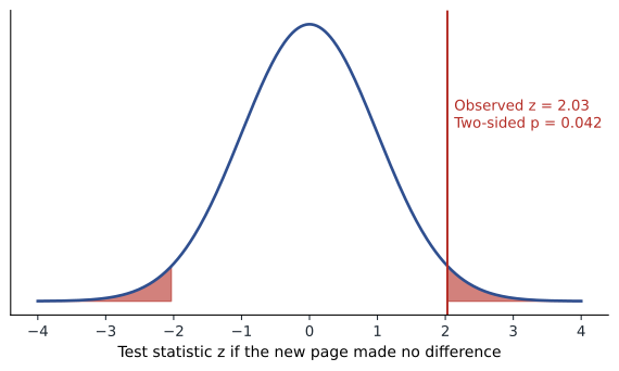
For Kestrel, the pooled rate is 856 out of 8,000, or 10.7 percent. The standard error is the square root of 0.107 times 0.893 times two divided by 4,000, about 0.0069. The observed difference of 0.014 is therefore about 2.03 standard errors. The p-value is the probability, assuming the null hypothesis is true, of seeing a difference at least this large in either direction. From the normal curve, that probability is about 0.042.
What a p-value does and does not mean
The p-value is one of the most misunderstood numbers in business and science, so it is worth being precise. A p-value of 0.042 means that if the new page truly made no difference, random assignment alone would produce a difference of 1.4 points or more, in either direction, about 4.2 percent of the time. It does not mean there is a 4.2 percent chance that the null hypothesis is true, nor a 95.8 percent chance that the new page is better. It says nothing directly about how large or important the effect is. The American Statistical Association took the unusual step in 2016 of publishing a statement warning against these misreadings and against treating 0.05 as a bright line between real and unreal effects.
Conventionally, results with a p-value below 0.05 are called statistically significant. The threshold, called the significance level, is a convention, not a law of nature. A manager deciding whether to change a web page that can be switched back in minutes might reasonably act on weaker evidence. A hospital deciding whether to change a clinical protocol might demand much stronger evidence. What matters is to set the threshold before looking at the data, in light of the costs of being wrong, and to report the p-value and the size of the effect rather than just a verdict.
Two kinds of error
A test can go wrong in two ways. A Type I error, or false positive, occurs when the test declares a difference that is not real; its probability, when the null is true, equals the significance level. A Type II error, or false negative, occurs when a real difference goes undetected. The power of a test is the probability of detecting a real effect of a given size, which is one minus the probability of a Type II error. Power depends on the size of the effect, the sample size, the variability of the outcome and the significance level.
| No real difference | Real difference | |
|---|---|---|
| Test says significant | Type I error (false positive) | Correct detection (power) |
| Test says not significant | Correct | Type II error (false negative) |
Many business experiments are badly underpowered: they run on too few customers to have a reasonable chance of detecting the modest effects that most changes produce. A non-significant result from an underpowered test says little; the effect might be zero or might be valuable but hidden in the noise. Dr. Zhou's rule is to calculate power before running a test, and to report a confidence interval for the effect afterwards, so that readers can see which effect sizes the data rule out and which they do not.
Effect size and confidence intervals
Rather than just a p-value, a manager should look at an interval for the difference. Using the unpooled standard error, about 0.0069, a 95 percent interval for the improvement is 1.4 points plus or minus 1.35, or roughly 0.05 to 2.75 points. The new page probably helps, but the improvement could be as small as a twentieth of a point or nearly three points. In business terms, Kestrel gets about 30,000 trial-page visitors a month; at the point estimate the new page would add about 420 trials a month, and at the bottom of the interval only about 15. Whether that matters depends on how many trials turn into paying customers and what those customers are worth.
This is the distinction between statistical and practical significance. With a very large sample, a trivial difference can be highly significant; with a small sample, an important difference may not reach significance. The decision should rest on the plausible range of the effect and its value, compared with the cost and risk of the change. For a page redesign that costs nothing to keep, the case for adopting it is strong. For a change that requires rebuilding an onboarding process, Leo might want more evidence first.
# Two-proportion z test and confidence interval for Kestrel's A/B test
import math
from statistics import NormalDist
nA, xA = 4000, 400      # current page
nB, xB = 4000, 456      # new page
pA, pB = xA / nA, xB / nB
pooled = (xA + xB) / (nA + nB)
se0 = math.sqrt(pooled * (1 - pooled) * (1 / nA + 1 / nB))
z = (pB - pA) / se0
p_value = 2 * (1 - NormalDist().cdf(abs(z)))
se1 = math.sqrt(pA * (1 - pA) / nA + pB * (1 - pB) / nB)
lo, hi = (pB - pA) - 1.96 * se1, (pB - pA) + 1.96 * se1
print(f"Rates: A {pA:.1%}, B {pB:.1%}, difference {pB - pA:.2%}")
print(f"z = {z:.2f}, two-sided p = {p_value:.3f}")
print(f"95% interval for the difference: {lo:.2%} to {hi:.2%}")

# Visitors per group needed to detect 10% -> 11% with 80% power at the 5% level
za, zb = NormalDist().inv_cdf(0.975), NormalDist().inv_cdf(0.80)
p1, p2 = 0.10, 0.11
n = (za + zb) ** 2 * (p1 * (1 - p1) + p2 * (1 - p2)) / (p2 - p1) ** 2
print(f"Visitors needed per group: {math.ceil(n):,}")Rates: A 10.0%, B 11.4%, difference 1.40% z = 2.03, two-sided p = 0.043 95% interval for the difference: 0.05% to 2.75% Visitors needed per group: 14,749
The second calculation is a warning. To have an 80 percent chance of detecting an improvement from 10 to 11 percent, Kestrel would need about 14,700 visitors in each group, nearly four times as many as it used. Kestrel's test detected a difference partly because the observed effect happened to be on the larger side. Had the true effect been one point, the test would more likely than not have come back non-significant.
The trouble with peeking
A common mistake in online experiments is to check the results every day and stop as soon as the p-value dips below 0.05. Because p-values fluctuate as data accumulate, a test with no real effect will often cross the threshold at some point if it is checked often enough. Repeated peeking with stopping at the first significant result can push the false positive rate from five percent to well over 20 percent. The remedies are to fix the sample size in advance and analyze once, or to use sequential testing methods designed for continuous monitoring, which many experimentation platforms now offer.
# How peeking inflates false positives when there is no real effect
import math, random
from statistics import NormalDist
random.seed(7)
def z_stat(xa, na, xb, nb):
    p = (xa + xb) / (na + nb)
    se = math.sqrt(p * (1 - p) * (1 / na + 1 / nb))
    return 0 if se == 0 else (xb / nb - xa / na) / se
crit = NormalDist().inv_cdf(0.975)
experiments, false_once, false_end = 1000, 0, 0
for _ in range(experiments):
    xa = xb = na = nb = 0
    crossed = False
    for day in range(14):                 # 14 daily looks, 300 visitors per arm per day
        for _ in range(300):
            na += 1; xa += random.random() < 0.10
            nb += 1; xb += random.random() < 0.10   # same true rate in both arms
        if abs(z_stat(xa, na, xb, nb)) > crit:
            crossed = True
    false_once += crossed
    false_end += abs(z_stat(xa, na, xb, nb)) > crit
print(f"Significant at the final look only: {false_end / experiments:.1%}")
print(f"Significant at any of 14 daily looks: {false_once / experiments:.1%}")Significant at the final look only: 5.5% Significant at any of 14 daily looks: 23.2%
Running good business experiments
Dr. Zhou gives the cohort a checklist drawn from practice at firms that experiment at scale. Choose one primary metric in advance, tied to the decision, and a small number of guardrail metrics, such as page load time, refunds or complaints, that must not get worse. Calculate the sample size needed for the smallest effect worth detecting. Randomize at the right level: by customer rather than by visit if the same person may return, and by store or region if customers interact or prices must be consistent. Check that the groups received the intended traffic split; a large mismatch, called a sample ratio mismatch, often signals a technical fault. Run the test for whole weeks to cover weekday and weekend behavior. And be wary of novelty effects, where users react to anything new at first and then return to old habits.
Experiments are not limited to websites. Grace has tested shelf layouts by randomly assigning matched stores to new and old layouts. Hana's clinics have tested text-message appointment reminders by randomizing patients, a kind of intervention that has been evaluated in many health systems with reductions in missed appointments. Daniel could randomize which production cells receive a new maintenance schedule. Where randomization is impossible or unethical, the methods in lesson 7 help, but they rely on stronger assumptions.
Worked problem
Planning a reminder experiment at Lakeview
Lakeview's clinics have a missed-appointment rate of about 12 percent. Hana wants to test a new two-day text reminder and would act if it cut missed appointments to 10 percent or lower. How many patients are needed in each arm for 80 percent power at the 5 percent level?
Show solution
- Identify the rates: p1 = 0.12 for usual care, p2 = 0.10 for reminders, a difference of 0.02.
- Compute the variance terms: 0.12 times 0.88 = 0.1056 and 0.10 times 0.90 = 0.09, sum 0.1956.
- Apply the formula: n = (1.96 + 0.84) squared times 0.1956 divided by 0.02 squared = 7.84 times 0.1956 / 0.0004.
- Calculate: 7.84 times 0.1956 = 1.5335; divided by 0.0004 gives about 3,834 patients per arm.
Answer: Hana needs about 3,800 patients in each arm, or roughly 7,700 appointments in total. With about 2,000 appointments a week across the clinics, the trial can be completed in about four weeks, randomizing by patient so that each person always receives the same treatment.
Common mistakes
MistakeA p-value of 0.04 means there is a 4 percent chance the change had no effect.
InsteadIt is the probability of data this extreme if there were no effect, not the probability that there is no effect.
MistakeA non-significant result proves there is no effect.
InsteadAn underpowered test may miss a real effect; look at the confidence interval.
MistakeStatistical significance means the effect is important.
InsteadJudge the size and value of the effect, not just whether p is below 0.05.
MistakeIt is fine to stop an experiment as soon as it becomes significant.
InsteadRepeated peeking inflates false positives; fix the sample size or use sequential methods.
Summary and key terms
- Random assignment makes groups alike on average, so differences can be attributed to the change or to chance.
- A hypothesis test asks how surprising the data would be if there were no effect; the p-value measures that surprise.
- Balance Type I and Type II errors, and calculate power and sample size before testing.
- Report a confidence interval for the effect and judge practical as well as statistical significance.
- Avoid peeking, define primary and guardrail metrics in advance, and check the traffic split.
- Null hypothesis
- The assumption that a change has no effect, which a test tries to find evidence against.
- p-value
- The probability of a result at least as extreme as the one observed, if the null hypothesis were true.
- Significance level
- The threshold below which a p-value is treated as evidence against the null, often 0.05.
- Type I error
- Declaring an effect that is not real.
- Type II error
- Failing to detect an effect that is real.
- Power
- The probability that a test detects an effect of a given size.
Practice problems
Work each problem on paper first, then reveal the answer to check.
In an A/B test, version A converts 300 of 5,000 visitors and version B converts 350 of 5,000. Compute the z statistic.
Show answer
Pooled rate = 650 / 10,000 = 0.065. SE = square root of 0.065 times 0.935 times 2 / 5,000 = 0.00493. Difference = 0.01, so z is about 2.03.
Why should an experiment be randomized by customer rather than by page view?
Show answer
The same customer may visit several times; randomizing by view could show them both versions and mix the effects, and views from one person are not independent.
An experiment finds no significant difference, with a 95 percent interval for the effect from minus 1 to plus 4 points. What can you conclude?
Show answer
The data are consistent with no effect but also with a useful gain of up to 4 points; the test was not precise enough to rule out a valuable effect.
An online test planned a 50/50 split but recorded 52,000 users in one group and 48,000 in the other. What should the analyst check?
Show answer
A sample ratio mismatch of this size is very unlikely by chance; check for bugs in assignment, logging or redirects before trusting the results.
Lesson quiz · 5 questions
Score 60% or more to complete this lesson.
Create a free account to save your progress, take quizzes and earn a certificate.