
GEOM-320 · Lesson 9 of 12 · 23 min
Radar and InSAR
Where the canal runs along the top of the coulee, two stretches of the bank had shown tension cracks in the first spring, and the district's geotechnical consultant had installed two inclinometers and asked whether the slope movement could be watched over a wider area. Ground surveys of monitoring points every three months were possible but expensive, and they could not cover the full 24 km. Ruth suggested radar interferometry, which can measure ground movement of a few millimeters per year over large areas from satellites that see through cloud and darkness. NISAR's L-band radar, with a 12-day repeat and newly public interferometric products, and Sentinel-1 offered the data. This lesson explains how imaging radar works, how radar images are formed and interpreted, and how interferometry turns the phase of radar echoes into maps of topography and ground deformation.
Imaging radar
A radar transmits pulses of microwave radiation and records the echoes. Imaging radars on satellites look to one side of the ground track, at incidence angles typically between 20° and 50°, because a radar looking straight down could not tell apart echoes from points at equal distance on both sides. The direction of flight is called azimuth and the direction across track, along the line of sight, is called range. Position in range is determined by the time delay of the echo; the slant range resolution is set by the bandwidth \(B\) of the transmitted pulse, \(\delta_r = c/(2B)\), and is projected onto the ground as \(\delta_g = \delta_r / \sin\theta\), where \(\theta\) is the incidence angle. A 50 MHz chirp gives 3 m in slant range and about 5 m on the ground at 35°.
Resolution in azimuth would be poor for a real antenna, since the beam footprint of a 12 m antenna at 700 km range is several kilometers long. Synthetic aperture radar (SAR) overcomes this by recording the echoes of each ground point during the whole time it is in the beam and processing them coherently, using the Doppler shift caused by the platform's motion, as if they had been received by an antenna as long as the distance flown. The resulting azimuth resolution in stripmap mode is about half the physical antenna length, independent of range. Other modes trade resolution for swath: ScanSAR and TOPS modes cover 250 to 500 km swaths at coarser resolution, while spotlight modes steer the beam to dwell on a small area for sub-meter resolution.
| Band | Frequency | Wavelength | Examples | Characteristics |
|---|---|---|---|---|
| X | About 8 to 12 GHz | About 3 cm | Commercial constellations | Fine detail; interacts with leaves; low coherence over vegetation |
| C | About 4 to 8 GHz | About 5.5 cm | Sentinel-1, RADARSAT Constellation Mission | Widely used for floods, ice and agriculture |
| S | About 2 to 4 GHz | About 9 cm | NISAR S-band | Intermediate penetration |
| L | About 1 to 2 GHz | About 24 cm | NISAR L-band, ALOS-2 | Penetrates vegetation; keeps coherence longer |
| P | About 0.4 GHz | About 70 cm | ESA Biomass | Forest biomass |
What controls radar brightness
The strength of the echo from a surface, expressed as the backscatter coefficient \(\sigma^0\) and usually given in decibels, depends on the radar's wavelength, polarization and incidence angle and on the surface's roughness, geometry and dielectric constant. Roughness is judged relative to the wavelength: a surface with irregularities much smaller than the wavelength acts as a mirror and reflects the pulse away, so calm water, smooth asphalt and the canal appear dark. Rough surfaces scatter in all directions and return part of the energy. Vegetation produces volume scattering from leaves, stems and branches. Corners formed by two perpendicular surfaces, such as a wall and the ground or the canal check structures, return energy directly to the radar by double bounce and appear very bright; deliberately installed metal corner reflectors use this effect to provide stable targets for interferometry.
The dielectric constant of most dry natural materials is low, about 3 to 8, while that of water is about 80. Moisture in soil and vegetation therefore raises backscatter strongly, which allows radar to track soil moisture and irrigation, and freshly irrigated fields often appear bright in C-band images. Polarization describes the orientation of the transmitted and received waves: HH and VV are co-polarized, HV and VH cross-polarized. Cross-polarized returns come mainly from multiple scattering in vegetation volumes and are a good indicator of biomass; co-polarized returns are stronger from surfaces and double bounce. Flooded vegetation, such as cattails standing in water, gives very strong HH returns by double bounce between the water and the stems, the opposite of open water.
Geometry and speckle
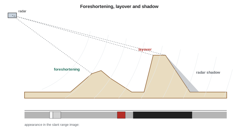
Because radar measures distance, relief produces distortions quite different from optical images. Slopes facing the radar are compressed in range, an effect called foreshortening, and appear bright because many scatterers fall into few pixels. If a slope is steeper than the incidence angle, its top is closer to the radar than its foot and is imaged before it, an effect called layover. Slopes facing away from the radar that are steeper than the complement of the incidence angle are not illuminated at all and appear as radar shadow. The coulee banks, with slopes of 25° to 35°, produced foreshortening on ascending passes and near-shadow on descending passes for some sections, which mattered when choosing the geometry for monitoring.
Radar images have a grainy texture called speckle. Each resolution cell contains many scatterers whose echoes add coherently with random phases, so the recorded intensity varies strongly from pixel to pixel even over a uniform field. Speckle is not noise in the sense of a sensor error, but for interpreting brightness it behaves like multiplicative noise. Averaging \(N\) independent looks, either by multilooking in processing or by spatial filtering, reduces the relative standard deviation of intensity as \(1/\sqrt{N}\) at the cost of resolution. Adaptive filters such as the Lee and refined Lee filters smooth uniform areas while preserving edges and bright points.
Interferometry
A SAR image is complex: each pixel records an amplitude and a phase. The phase depends on the distance from the antenna to the scatterers, modulo one wavelength, and on the scattering properties of the cell. On its own the phase of one image looks random. But if two images of the same area are acquired from nearly the same position at different times, and the scatterers in each cell have not changed, the random part cancels when one image is multiplied by the complex conjugate of the other, leaving an interferogram whose phase difference reflects the difference in range. A change in range of half a wavelength produces a full cycle of phase, because the signal travels the path twice:
For C-band, with a wavelength of 5.55 cm, one fringe of \(2\pi\) corresponds to 27.7 mm of range change; for L-band at 24 cm, about 120 mm. The sign convention varies between processing systems and must always be checked; here a positive phase change corresponds to an increase in range, motion away from the satellite.
The interferometric phase has several components: a flat-Earth phase from the change of viewing geometry across the scene, which is removed with the orbits; a topographic phase proportional to the perpendicular baseline between the two orbits, which is removed with a DEM or, in a single-pass system such as the TanDEM-X pair, used to make the DEM; a deformation phase from ground movement along the line of sight; an atmospheric phase from differences in water vapor between the two dates, which can amount to a few centimeters and is the main limit on accuracy; and noise. The quality of the interferogram is measured by coherence, between 0 and 1, which falls when scatterers change between the dates. Water and actively cultivated fields lose coherence within days at C-band; grassland keeps it for weeks; rock, buildings and bare stable soil for months or years. Longer wavelengths keep coherence better over vegetation.
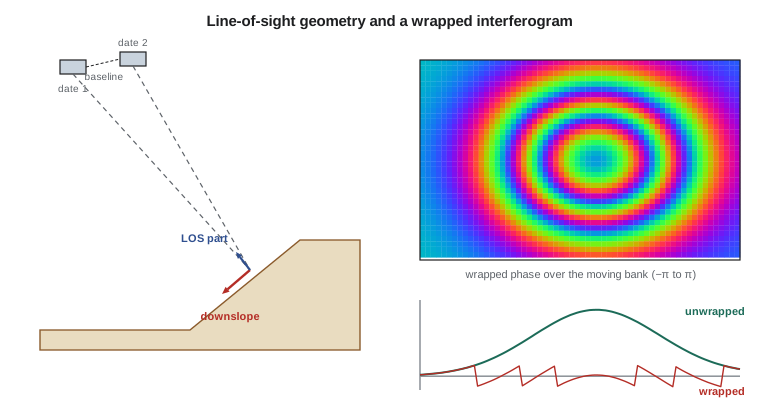
The measured phase is wrapped into the interval from \(-\pi\) to \(\pi\). Phase unwrapping restores the integer number of cycles by integrating phase differences between neighboring pixels, assuming that the true difference between neighbors is less than half a cycle. Unwrapping fails where coherence is low or deformation is steep, producing errors of whole cycles that propagate along the unwrapping path. Persistent scatterer and small baseline time series methods process stacks of tens or hundreds of images, select pixels with stable scattering and estimate deformation histories and velocities while separating atmospheric effects, which vary randomly from date to date, from deformation, which is correlated in time. With long stacks, line-of-sight velocities can be estimated to a millimeter or two per year.
import math
c = 2.99792458e8
# Wavelengths of the radars used in the course
for name, f_ghz in (("RCM / Sentinel-1 (C-band)", 5.405), ("NISAR L-band", 1.257), ("NISAR S-band", 3.2), ("X-band commercial", 9.65)):
    print(f"{name:26s} {f_ghz:6.3f} GHz  wavelength {c / (f_ghz * 1e9) * 100:5.2f} cm")

# Resolution of a SAR: slant range from bandwidth, ground range from incidence, azimuth from antenna length
B, inc, L = 50e6, 35.0, 12.0
dr = c / (2 * B)
print(f"\nslant range resolution {dr:.1f} m, ground range {dr / math.sin(math.radians(inc)):.1f} m at {inc} deg incidence")
print(f"stripmap azimuth resolution about L/2 = {L / 2:.1f} m, independent of range")

# Speckle: averaging N looks reduces the relative standard deviation of intensity as 1/sqrt(N)
for N in (1, 4, 16, 49):
    print(f"{N:3d} looks: relative sd of intensity {1 / math.sqrt(N):.2f}")

# Interferometric phase to line-of-sight displacement
lam = c / 5.405e9
print()
for dphi in (math.pi / 4, math.pi, 2 * math.pi):
    print(f"phase change {dphi:5.3f} rad -> LOS displacement {-lam * dphi / (4 * math.pi) * 1000:6.2f} mm")

# Unwrap a wrapped phase profile across the coulee bank (radians, 12-day pairs stacked)
wrapped = [0.2, 0.9, 1.7, 2.6, -2.9, -2.1, -1.2, -0.5, 0.3, 1.1, 1.8]
unw = [wrapped[0]]
for w in wrapped[1:]:
    step = w - wrapped[len(unw) - 1]
    step -= 2 * math.pi * round(step / (2 * math.pi))
    unw.append(unw[-1] + step)
print("\nunwrapped phase:", " ".join(f"{u:5.2f}" for u in unw))
print("LOS displacement (mm):", " ".join(f"{-lam * u / (4 * math.pi) * 1000:5.1f}" for u in unw))

# Time series of one persistent scatterer on the bank: LOS displacement (mm) every 24 days
t = [0, 24, 48, 72, 96, 120, 144, 168, 192, 216]
dlos = [0.0, -1.1, -2.6, -3.1, -4.9, -5.6, -6.2, -7.9, -8.4, -9.8]
n = len(t); mt = sum(t) / n; md = sum(dlos) / n
v = sum((a - mt) * (b - md) for a, b in zip(t, dlos)) / sum((a - mt) ** 2 for a in t)
res = [b - (md + v * (a - mt)) for a, b in zip(t, dlos)]
s = math.sqrt(sum(r * r for r in res) / (n - 2))
print(f"\nLOS velocity {v * 365.25:.1f} mm/yr, residual sd {s:.2f} mm")
# If the motion is downslope on a bank facing the satellite, LOS sees only the component along the look direction
theta = math.radians(38.0)
print(f"pure vertical motion would be {v * 365.25 / math.cos(theta):.1f} mm/yr at 38 deg incidence")RCM / Sentinel-1 (C-band) 5.405 GHz wavelength 5.55 cm NISAR L-band 1.257 GHz wavelength 23.85 cm NISAR S-band 3.200 GHz wavelength 9.37 cm X-band commercial 9.650 GHz wavelength 3.11 cm slant range resolution 3.0 m, ground range 5.2 m at 35.0 deg incidence stripmap azimuth resolution about L/2 = 6.0 m, independent of range 1 looks: relative sd of intensity 1.00 4 looks: relative sd of intensity 0.50 16 looks: relative sd of intensity 0.25 49 looks: relative sd of intensity 0.14 phase change 0.785 rad -> LOS displacement -3.47 mm phase change 3.142 rad -> LOS displacement -13.87 mm phase change 6.283 rad -> LOS displacement -27.73 mm unwrapped phase: 0.20 0.90 1.70 2.60 3.38 4.18 5.08 5.78 6.58 7.38 8.08 LOS displacement (mm): -0.9 -4.0 -7.5 -11.5 -14.9 -18.5 -22.4 -25.5 -29.1 -32.6 -35.7 LOS velocity -16.2 mm/yr, residual sd 0.30 mm pure vertical motion would be -20.6 mm/yr at 38 deg incidence
The unwrapping example shows the profile across a moving section of the bank. The wrapped values jump from 2.6 to −2.9 radians, but the unwrapped profile recognizes that the true step is +0.78 radians and continues smoothly to 8.1 radians, about 36 mm of range change across the section. The persistent scatterer time series, on a concrete outlet structure on the bank, gives a line-of-sight velocity of about −16 mm per year with residuals of only 0.3 mm, a clear signal of movement.
From line of sight to ground motion
InSAR measures only the component of motion along the line of sight, which for a right-looking satellite on an ascending or descending pass points toward the satellite at the incidence angle, roughly from the east or the west. Vertical motion projects onto the line of sight by \(\cos\theta\), east-west motion by about \(\sin\theta\), and north-south motion almost not at all, because near-polar orbits look nearly east or west. The bank sections that worried the consultant faced north-east and south-west across the coulee, so their downslope motion had a large east-west component. Combining ascending and descending geometries allows the vertical and east-west components to be separated, and assuming that motion is parallel to the local slope gives an estimate of the downslope rate.
Worked problem
Converting line-of-sight velocity
A persistent scatterer has a line-of-sight velocity of −16.2 mm per year at an incidence angle of 38°. If the motion were purely vertical, what would the vertical rate be? If instead the motion were purely east-west and the satellite looks toward the east, what horizontal rate would explain it?
Show solution
- \[v_{vert} = \frac{-16.2}{\cos 38°} = \frac{-16.2}{0.788} = -20.6 \text{ mm/yr}\]
- \[v_{EW} = \frac{-16.2}{\sin 38°} = \frac{-16.2}{0.616} = -26.3 \text{ mm/yr}\]
Answer: The same line-of-sight measurement is consistent with 21 mm per year of subsidence or 26 mm per year of horizontal motion away from the satellite. A second viewing geometry, or knowledge of the slope direction, is needed to decide.
The program adopted monthly processing of NISAR L-band stacks over the canal corridor, with Sentinel-1 as a cross-check, and three corner reflectors installed by Grant's crew on stable ground and on the two moving sections to provide reference points that remain coherent through the growing season. The InSAR results, the inclinometers and RTK surveys of the reflectors twice a year would be compared at every report, so that the satellite measurements were tied to ground truth.
Common mistakes
MistakeInterpreting dark radar areas as dry or empty.
InsteadDark means little energy returned: smooth surfaces such as water or shadowed slopes.
MistakeReading every fringe in an interferogram as deformation.
InsteadRemove orbital and topographic phase and consider atmospheric delays before interpreting fringes.
MistakeReporting InSAR line-of-sight values as vertical movement.
InsteadState the geometry, combine passes or project with a stated assumption.
MistakeUsing C-band interferometry over growing crops for monthly intervals.
InsteadExpect coherence loss; use longer wavelengths, persistent scatterers or corner reflectors.
MistakeIgnoring the sign convention of the processing software.
InsteadCheck whether positive values mean motion toward or away from the satellite.
Summary and key terms
- Side-looking SAR resolves range by pulse bandwidth and azimuth by synthesizing a long aperture.
- Backscatter depends on wavelength, polarization, incidence angle, roughness, geometry and moisture.
- Foreshortening, layover and shadow distort radar images of slopes; speckle is reduced by multilooking and filtering.
- Interferometry uses the phase difference between two complex images: one fringe equals half a wavelength of range change.
- Interferometric phase contains flat-Earth, topographic, deformation, atmospheric and noise terms; coherence measures quality.
- Unwrapping restores whole cycles; time series methods estimate velocities to millimeters per year.
- InSAR measures line-of-sight motion; several geometries are needed to resolve components.
- Synthetic aperture radar
- An imaging radar that processes echoes along the flight path to synthesize a long antenna and fine azimuth resolution.
- Backscatter coefficient
- The normalized radar cross-section per unit ground area, usually in decibels.
- Layover
- A radar distortion in which the top of a steep slope is imaged before its foot.
- Speckle
- The granular interference pattern in coherent radar images.
- Interferogram
- An image of the phase difference between two complex SAR images.
- Coherence
- A measure from 0 to 1 of the similarity of scattering between two SAR acquisitions.
- Line of sight
- The direction from the ground to the radar antenna, along which InSAR measures motion.
Practice problems
Work each problem on paper first, then reveal the answer to check.
What slant range resolution does a 100 MHz bandwidth give?
Show answer
c/(2B) = 3 × 10⁸ / 2 × 10⁸ = 1.5 m.
How much line-of-sight displacement does one fringe represent at L-band with λ = 23.8 cm?
Show answer
λ/2 = 11.9 cm.
A phase change of 1.5 rad is measured at C-band (5.55 cm). What is the range change?
Show answer
0.0555 × 1.5 / (4π) = 6.6 mm.
How many looks reduce the relative standard deviation of speckle to 0.2?
Show answer
1/√N = 0.2, so N = 25.
Why does open water appear dark in radar images?
Show answer
It acts as a mirror and reflects the pulse away from the antenna.
Lesson quiz · 5 questions
Score 60% or more to complete this lesson.
Create a free account to save your progress, take quizzes and earn a certificate.