Classification

The board's first concrete request was a map of what was growing in every field in the service area that summer, with the area of each crop, to compare with the water orders. The district had water orders by field but no reliable record of the crops, and the provincial and national crop maps were released months after the season and did not always match the district's field boundaries. Leah's team would produce their own map from Sentinel-2 and Landsat images, check it against field visits and state its accuracy. This lesson explains how images are classified into thematic maps: the training data, the unsupervised and supervised classifiers, object-based methods, and the accuracy assessment and area estimation that make a map trustworthy.

What classification does

Classification assigns each pixel, or each object such as a field, to one of a set of classes on the basis of its spectral, temporal, spatial or contextual properties. The result is a thematic map: crop types, land cover, irrigated and non-irrigated land, water and not water. Every classification starts with a legend, the list of classes with definitions that are mutually exclusive and cover everything in the area. A legend that includes alfalfa and forage without saying how to tell them apart, or that has no class for farmyards, will produce confusion that no algorithm can fix. The district's legend had ten classes: alfalfa, spring wheat, durum or winter wheat, barley, canola, potatoes, sugar beets or other row crops, grass and pasture, fallow and bare soil, and water, with roads and farmyards assigned to an eleventh class, developed.

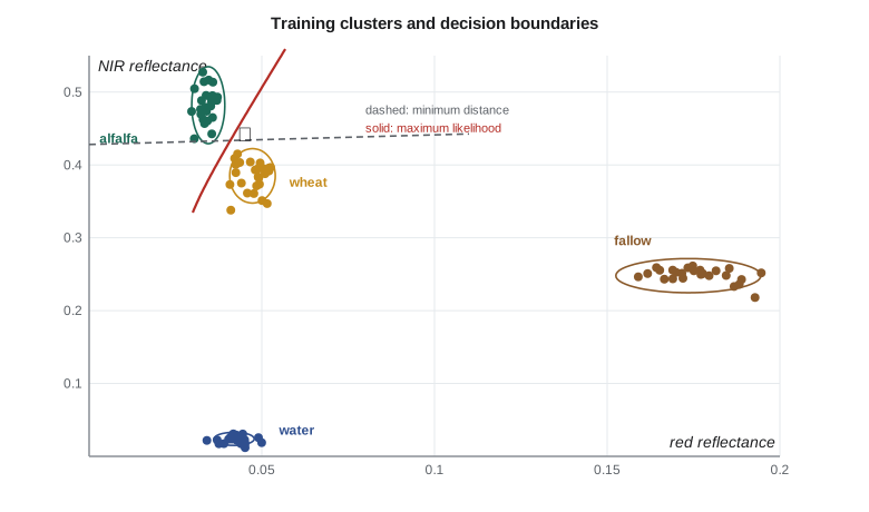
Pixels are classified in a feature space whose axes are the variables used: band reflectances, indices, values from several dates, texture measures or radar backscatter. Each class occupies a region of that space, and a classifier is a rule that divides the space into regions, one per class. Classes are separable if their regions overlap little. The spectral angles of Lesson 2 already showed that on one July date alfalfa, wheat and canola overlap strongly, while green crops, bare soil and water separate well.

Unsupervised classification

Unsupervised classification groups pixels into spectral clusters without prior knowledge of the classes; the analyst then labels the clusters. The k-means algorithm starts with k cluster centers, assigns each pixel to the nearest center, recomputes each center as the mean of its pixels, and repeats until the assignments stop changing. ISODATA adds rules to split clusters with large spread and merge clusters that are close. Unsupervised methods are useful for exploring an image, finding classes the analyst did not anticipate, and stratifying an area for sampling. Their weakness is that spectral clusters do not necessarily correspond to information classes: one crop may split into several clusters by soil type or growth stage, and two crops may fall into one cluster. Labeling the clusters requires the same field knowledge that supervised methods use from the start.

Training data

Supervised classification learns from training samples of known class. The quality of the samples matters more than the choice of algorithm. Samples must be representative of the variation within each class across the whole area: different soils, sowing dates, irrigation methods and field conditions. They must be correctly labeled, and labels from farmers, crop insurance records or field visits must be checked for the right year and field. They must be numerous enough to estimate the class statistics, with a common rule of at least 10 to 30 times as many pixels as features for statistical classifiers, and in practice many fields per class rather than many pixels from a few fields. And they must be independent of the samples later used for accuracy assessment.

Grant's crew visited about 300 fields during the season, chosen by a stratified random design from the district's field list, recording the crop and its condition with geotagged photographs. Half of the fields, chosen at random, were set aside for validation before any classification was done. Pixels at field edges were excluded from training with a 20 m inward buffer to avoid mixed pixels.

Supervised classifiers

The minimum-distance classifier assigns each pixel to the class whose mean is nearest in feature space. It is simple and fast but ignores the spread of each class, so a class with a wide spread, such as fallow on varied soils, loses pixels to a compact neighbor. The parallelepiped classifier assigns a pixel to a class if it falls within a box defined by the minimum and maximum, or the mean plus or minus a few standard deviations, of the training values in each feature; it is fast but leaves pixels unclassified outside all boxes and ambiguous where boxes overlap.

The Gaussian maximum likelihood classifier models each class as a multivariate normal distribution with its own mean vector \(\mathbf{m}_k\) and covariance matrix \(\mathbf{S}_k\), and assigns a pixel \(\mathbf{x}\) to the class with the largest discriminant function:

where \(p(k)\) is the prior probability of the class. The quadratic term is the squared Mahalanobis distance, which measures distance in units of the class's own spread along each direction. Maximum likelihood accounts for the different shapes of classes and gives curved decision boundaries. It needs enough training pixels to estimate each covariance matrix, it assumes normal distributions that real classes, especially multimodal ones, may not follow, and it degrades when there are many correlated features. Machine learning classifiers, which avoid these assumptions, are the subject of Lesson 11.

import math
# Training pixels (red reflectance, NIR reflectance) digitized from fields checked by the crew
train = {
    "alfalfa": [(0.034, 0.47), (0.036, 0.50), (0.031, 0.45), (0.038, 0.49), (0.033, 0.46), (0.035, 0.52)],
    "wheat":   [(0.046, 0.39), (0.050, 0.37), (0.043, 0.41), (0.048, 0.36), (0.045, 0.40), (0.052, 0.38)],
    "fallow":  [(0.170, 0.25), (0.182, 0.24), (0.165, 0.26), (0.176, 0.23), (0.160, 0.25), (0.188, 0.26)],
    "water":   [(0.040, 0.020), (0.044, 0.025), (0.038, 0.018), (0.046, 0.030), (0.041, 0.022), (0.043, 0.027)],
}
stats = {}
for k, pts in train.items():
    n = len(pts)
    m = [sum(p[i] for p in pts) / n for i in (0, 1)]
    v = [sum((p[i] - m[i]) ** 2 for p in pts) / (n - 1) for i in (0, 1)]
    stats[k] = (m, v)
    print(f"{k:8s} mean red {m[0]:.4f} NIR {m[1]:.3f}   sd red {math.sqrt(v[0]):.4f} NIR {math.sqrt(v[1]):.4f}")

def min_dist(x):
    return min(stats, key=lambda k: (x[0] - stats[k][0][0]) ** 2 + (x[1] - stats[k][0][1]) ** 2)
def max_like(x):   # Gaussian with independent bands, equal priors
    def g(k):
        m, v = stats[k]
        return -sum(math.log(v[i]) + (x[i] - m[i]) ** 2 / v[i] for i in (0, 1))
    return max(stats, key=g)

x = (0.045, 0.44)
print(f"\npixel {x}: minimum distance -> {min_dist(x)}, maximum likelihood -> {max_like(x)}")

# Accuracy assessment: rows = map class, columns = reference class (stratified random sample, 300 points)
cls = ["alfalfa", "wheat", "fallow", "water"]
E = [[52, 9, 1, 0],
     [7, 81, 4, 0],
     [2, 6, 118, 1],
     [0, 0, 2, 17]]
n = sum(map(sum, E))
diag = sum(E[i][i] for i in range(4))
oa = diag / n
print(f"\noverall accuracy {oa:.3f}")
for i, c in enumerate(cls):
    ua = E[i][i] / sum(E[i]); pa = E[i][i] / sum(E[r][i] for r in range(4))
    print(f"{c:8s} user's accuracy {ua:.3f}  producer's accuracy {pa:.3f}")
pe = sum(sum(E[i]) * sum(E[r][i] for r in range(4)) for i in range(4)) / n**2
print(f"kappa {(oa - pe) / (1 - pe):.3f} (chance agreement {pe:.3f})")

# Area estimation from the error matrix (stratified estimator)
mapped_ha = {"alfalfa": 6120.0, "wheat": 9480.0, "fallow": 12850.0, "water": 1550.0}
total = sum(mapped_ha.values())
W = [mapped_ha[c] / total for c in cls]
print("\nclass     mapped ha   estimated ha   95 % interval")
for j, c in enumerate(cls):
    p = sum(W[i] * E[i][j] / sum(E[i]) for i in range(4))
    var = sum(W[i] ** 2 * (E[i][j] / sum(E[i])) * (1 - E[i][j] / sum(E[i])) / (sum(E[i]) - 1) for i in range(4))
    print(f"{c:8s} {mapped_ha[c]:9.0f}  {p * total:11.0f}    +/- {1.96 * math.sqrt(var) * total:5.0f}")

alfalfa  mean red 0.0345 NIR 0.482   sd red 0.0024 NIR 0.0264
wheat    mean red 0.0473 NIR 0.385   sd red 0.0033 NIR 0.0187
fallow   mean red 0.1735 NIR 0.248   sd red 0.0105 NIR 0.0117
water    mean red 0.0420 NIR 0.024   sd red 0.0029 NIR 0.0045

pixel (0.045, 0.44): minimum distance -> alfalfa, maximum likelihood -> wheat

overall accuracy 0.893
alfalfa  user's accuracy 0.839  producer's accuracy 0.852
wheat    user's accuracy 0.880  producer's accuracy 0.844
fallow   user's accuracy 0.929  producer's accuracy 0.944
water    user's accuracy 0.895  producer's accuracy 0.944
kappa 0.843 (chance agreement 0.320)

class     mapped ha   estimated ha   95 % interval
alfalfa       6120         6057    +/-   815
wheat         9480         9842    +/-   958
fallow       12850        12613    +/-   758
water         1550         1488    +/-   296

The pixel with red 0.045 and NIR 0.44 shows the difference between the two rules. Its NIR value is a little closer to the alfalfa mean, and because the NIR differences are larger in absolute terms than the red differences, the minimum-distance rule chooses alfalfa. But its red value lies more than four alfalfa standard deviations from the alfalfa mean and less than one from the wheat mean, so maximum likelihood, which measures distance in units of each class's spread, chooses wheat. Minimum distance on raw reflectance implicitly weights bands by their range, which is rarely what the analyst intends.

Object-based classification

Pixel-based classification of 10 m imagery over large fields often produces a salt-and-pepper pattern of isolated misclassified pixels within fields. Object-based image analysis first segments the image into objects, groups of adjacent pixels that are similar, and then classifies the objects using their mean spectra, shape, texture and context. In the service area, the district's own field boundaries could serve as objects: every pixel inside a field boundary, buffered inward, would be averaged and the field classified as a whole, which matched the way water was ordered. Fields split between two crops were flagged when their pixel classes disagreed. Where boundaries are not available, segmentation algorithms group pixels by spectral similarity at a chosen scale, and the choice of scale, too fine or too coarse, strongly affects the result.

Accuracy assessment

A map without an accuracy statement is not finished. Accuracy is assessed by comparing the map with reference data at sample locations chosen by a probability sampling design, usually stratified random sampling with the map classes as strata, so that rare classes are adequately sampled. The comparison is summarized in a confusion matrix, or error matrix, with map classes as rows and reference classes as columns. Overall accuracy is the proportion of samples correctly classified, the sum of the diagonal divided by the total. User's accuracy for a class is the proportion of samples mapped as that class that really are that class; its complement is the commission error, and it tells a map user how reliable the label on the map is. Producer's accuracy is the proportion of reference samples of a class that were mapped correctly; its complement is the omission error, and it tells the map maker how well the class was found.

The kappa coefficient was long reported alongside overall accuracy as a measure of agreement beyond chance. It is now widely discouraged as a primary measure, because the chance agreement it subtracts is not a meaningful baseline for maps and because it adds nothing to the error matrix that overall, user's and producer's accuracies do not already say better. Good practice, as set out in widely cited guidance on accuracy assessment and area estimation, is to report the full error matrix, overall, user's and producer's accuracies with confidence intervals, and the sampling design used.

Estimating areas

Counting pixels of each class on the map gives map areas, but because the map has errors, these are biased: commission errors add area and omission errors remove it. The error matrix from a probability sample allows an unbiased estimate. With stratified sampling by map class, the proportion of area in reference class \(j\) is estimated as \(\hat{p}_j = \sum_i W_i \, n_{ij}/n_{i\cdot}\), where \(W_i\) is the mapped area proportion of stratum \(i\), \(n_{ij}\) is the number of samples mapped as \(i\) and found to be \(j\), and \(n_{i\cdot}\) is the number of samples in stratum \(i\). The standard error follows from the stratified sampling formulas, giving a confidence interval for each area. In the code, the mapped wheat area of 9,480 ha is adjusted upward to an estimated 9,842 ha because more wheat was omitted from the wheat class than was committed into it, with a 95 % interval of about ±960 ha.

National products give a useful comparison. The Cropland Data Layer of the U.S. Department of Agriculture's National Agricultural Statistics Service maps crop types across the conterminous United States at 30 m resolution each year, using satellite imagery from several sensors and a decision tree classifier trained with farmers' reported crop data, and NASS publishes accuracy statistics by state and crop; finer 10 m versions have been introduced for some areas. Leah compared the district's map with the layer for the previous year and found close agreement for the major crops, with differences mostly in forage and pasture classes and along field edges, where the district's own boundaries gave the local map an advantage.