Change detection

Two kinds of change interested the district. The first was slow: the canal right-of-way, 60 m wide and 24 km long, was supposed to stay in grass, but the operations staff suspected that weeds were spreading on the spoil piles, that some neighbors were cultivating into the right-of-way and that a new turnout structure had cleared more ground than planned. The second was sudden: in late August a grass fire started by a spark from a swather burned along the canal bank and into a shelterbelt before the volunteer fire department stopped it, and the district needed a map of the burned area and its severity within a week. Both were questions of change detection. This lesson describes how change is detected and measured from images of different dates, the preprocessing it demands, the main methods, burn severity, time series approaches and how change maps are validated.

What makes change detection hard

Change detection compares images of the same place at different times to find where the surface has changed, what the change was and, sometimes, how much. The difficulty is that images differ for many reasons besides change on the ground: illumination and sun angle, atmosphere, sensor calibration, view angle, soil moisture after rain, growth stage of crops, snow and misregistration. A change detection method must separate the change of interest from all these nuisance differences. Most of the work is in preparation: choosing images from the same season and similar sun angle, preferably the same sensor or harmonized sensors; converting both to surface reflectance; masking cloud, shadow and snow in both; and registering them to a fraction of a pixel.

Misregistration is a common source of false change. If two images are offset by half a pixel, every boundary between contrasting covers, such as the canal edge or a road, produces a line of apparent change. For 10 m data a registration error of 0.2 pixel, 2 m, is a reasonable target, and change along sharp edges should be interpreted with caution even then. Phenology is the other great confounder in agriculture: a field compared between June and August changes in every band because the crop has grown or been harvested, not because of anything the district cares about. For the right-of-way, Leah chose images from the same week in successive Julys.

Image differencing and ratioing

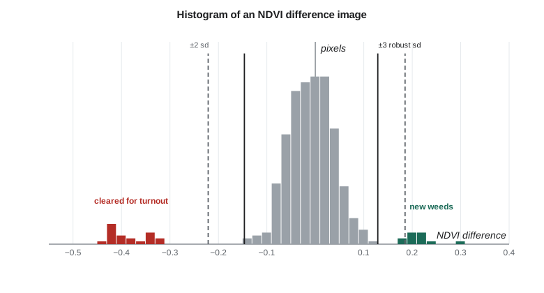
The simplest method subtracts one date from another, band by band or for an index such as NDVI, giving a difference image in which unchanged pixels cluster around zero and changed pixels lie in the tails. A threshold separates change from no change. A common choice is the mean of the difference image plus or minus a multiple of its standard deviation, with the multiple chosen to balance missed change against false alarms. Ratioing divides one date by the other and centers unchanged pixels on one; it is less sensitive to multiplicative illumination differences but behaves badly for dark targets.

The threshold is the critical decision. Changed pixels inflate the standard deviation of the difference image, so a threshold based on the ordinary standard deviation can be too wide and miss change, especially when a large share of the area has changed. Robust estimates of spread, such as the median absolute deviation, are less affected. Where reference data are available, the threshold can be tuned to the costs of the two kinds of error: for the right-of-way, a false alarm meant a wasted inspection visit, while a missed encroachment meant a dispute later, so the district preferred to accept some false alarms.

import math, random
random.seed(8)
# NDVI of 400 pixels along the canal right-of-way in two Julys (simulated from field-checked statistics)
n = 400
before = [random.gauss(0.52, 0.06) for _ in range(n)]
after = [b + random.gauss(0.0, 0.04) for b in before]
# 20 pixels cleared for the new turnout structure, 12 pixels of new weed growth on spoil piles
for i in range(100, 120): after[i] = random.gauss(0.14, 0.03)
for i in range(300, 312): after[i] = before[i] + random.gauss(0.22, 0.03)
d = [a - b for a, b in zip(after, before)]
m = sum(d) / n
s = math.sqrt(sum((x - m) ** 2 for x in d) / (n - 1))
print(f"difference image: mean {m:+.4f}, sd {s:.4f}")
for kk in (1.5, 2.0, 3.0):
    loss = [i for i, x in enumerate(d) if x < m - kk * s]
    gain = [i for i, x in enumerate(d) if x > m + kk * s]
    true_loss = set(range(100, 120)); true_gain = set(range(300, 312))
    fl = len([i for i in loss if i not in true_loss]); fg = len([i for i in gain if i not in true_gain])
    ml = len(true_loss - set(loss)); mg = len(true_gain - set(gain))
    print(f"k = {kk}: loss {len(loss):3d} (false {fl:2d}, missed {ml:2d})   gain {len(gain):3d} (false {fg:2d}, missed {mg:2d})")

# Robust threshold from the median and median absolute deviation
srt = sorted(d); med = srt[n // 2]
mad = sorted(abs(x - med) for x in d)[n // 2] * 1.4826
print(f"\nmedian {med:+.4f}, robust sd {mad:.4f} (the changed pixels inflate the ordinary sd)")
for kk in (2.0, 3.0):
    loss = [i for i, x in enumerate(d) if x < med - kk * mad]
    gain = [i for i, x in enumerate(d) if x > med + kk * mad]
    fl = len([i for i in loss if not 100 <= i < 120]); fg = len([i for i in gain if not 300 <= i < 312])
    print(f"robust k = {kk}: loss {len(loss):3d} (false {fl:2d})   gain {len(gain):3d} (false {fg:2d})")

# Burn severity from the differenced normalized burn ratio
def nbr(nir, swir2): return (nir - swir2) / (nir + swir2)
plots = {"grass verge, light burn": ((0.30, 0.18), (0.24, 0.20)),
         "shelterbelt, crown fire": ((0.38, 0.12), (0.12, 0.26)),
         "irrigated field, unburned": ((0.45, 0.10), (0.44, 0.10))}
print("\nplot                         NBR before  NBR after   dNBR")
for k, ((n1, s1), (n2, s2)) in plots.items():
    a, b = nbr(n1, s1), nbr(n2, s2)
    print(f"{k:28s} {a:8.3f}   {b:8.3f}   {a - b:6.3f}")

difference image: mean -0.0179, sd 0.1016
k = 1.5: loss  20 (false  0, missed  0)   gain  12 (false  0, missed  0)
k = 2.0: loss  20 (false  0, missed  0)   gain  12 (false  0, missed  0)
k = 3.0: loss  17 (false  0, missed  3)   gain   0 (false  0, missed 12)

median -0.0087, robust sd 0.0459 (the changed pixels inflate the ordinary sd)
robust k = 2.0: loss  25 (false  5)   gain  17 (false  5)
robust k = 3.0: loss  20 (false  0)   gain  12 (false  0)

plot                         NBR before  NBR after   dNBR
grass verge, light burn         0.250      0.091    0.159
shelterbelt, crown fire         0.520     -0.368    0.888
irrigated field, unburned       0.636      0.630    0.007

The simulated right-of-way has 400 pixels, of which 20 were cleared for the turnout and 12 developed new weeds. With the ordinary standard deviation of 0.10, inflated by the changed pixels, a threshold of 1.5 or 2 standard deviations finds all the changes without false alarms in this sample, but 3 standard deviations misses some cleared pixels and all the weed growth, whose NDVI increase of about 0.22 falls inside the threshold. The robust spread of 0.046 describes the unchanged pixels better: at 2 robust standard deviations the threshold catches all changes but adds 10 false alarms, while at 3 it is clean. In a real scene the unchanged pixels would not be perfectly normal and the right threshold would be checked against inspection results.

Other methods

Change vector analysis treats the differences in several bands, or in brightness and greenness, as a vector for each pixel. Its length measures the magnitude of change and its direction indicates the kind of change: loss of vegetation, gain of vegetation or a change in moisture. Principal component analysis of a stacked two-date image puts most of the unchanged variation in the first component and isolates change in later components, though the components must be interpreted for each scene. Post-classification comparison classifies each date separately and compares the maps, giving a full from-to matrix of change classes, such as grass to cultivated; its weakness is that the errors of both classifications compound, so two maps each 90 % accurate can give a change map with many false changes. Direct multidate classification classifies the stacked bands of both dates at once, using training samples of each change class.

Radar images can also be compared. The ratio of backscatter between two dates, or its logarithm, detects flooding, harvesting and construction, and the loss of interferometric coherence between dates, covered in the next lesson, is sensitive to any disturbance of the surface, including tillage that leaves reflectance almost unchanged. The district later used coherence loss to detect cultivation in the right-of-way during the cloudy spring months.

Burn severity

Fires lower near infrared reflectance, as green leaves are destroyed, and raise shortwave infrared reflectance, as the canopy opens, the soil dries and charcoal and ash are exposed. The normalized burn ratio captures both effects:

The difference between pre-fire and post-fire NBR, dNBR, increases with burn severity. Commonly used ranges, developed from field plots in forests of the western United States, classify dNBR below about 0.10 as unburned, 0.10 to 0.27 as low severity, 0.27 to 0.44 as moderate-low, 0.44 to 0.66 as moderate-high and above 0.66 as high severity. These ranges are a starting point and should be calibrated with field observations for each ecosystem; grasslands, which recover quickly and have little biomass, typically produce lower dNBR values than forests for a fire of similar intensity. The relative version, RdNBR, divides dNBR by a function of the pre-fire NBR so that sparse vegetation can still register high severity.

For large wildfires, national burned area products give a consistent record. In the United States, the Monitoring Trends in Burn Severity program maps the perimeters and dNBR-based severity of large fires from Landsat, and the national fire agencies provide perimeters and satellite hotspots. The district's fire was far too small for those products to describe in detail, so Leah mapped it herself from Sentinel-2 images a week before and three days after the fire, and Grant's crew visited 15 plots to calibrate the severity classes.

Time series approaches

Comparing two dates captures change between them but cannot distinguish a lasting change from a seasonal dip or a single bad image. With dense archives of Landsat and Sentinel-2 images, change can instead be detected in time series of every pixel. Methods such as LandTrendr fit piecewise linear trends to annual composites and identify breakpoints, such as a sudden loss followed by slow recovery after a fire. Methods such as CCDC, continuous change detection and classification, fit a harmonic model of the seasonal cycle and a trend to all clear observations and flag change when new observations depart from the model's prediction persistently; BFAST decomposes a series into trend, season and remainder and tests for breaks. Time series methods make full use of the archive, are less sensitive to the choice of dates and can give the timing of change, but they need consistently processed data and careful handling of cloud gaps and sensor differences.

For the right-of-way, Theo built a seasonal model of NDVI for each pixel from four years of Sentinel-2 data and set the program to flag any pixel whose observations fell below the model for three consecutive clear dates during the growing season. That rule caught a neighbor's cultivation within three weeks of its happening, while ignoring the brief dips after the right-of-way was mowed.

Validating change

Change maps are validated like classifications, with a probability sample and an error matrix, but with two practical complications. Change is usually rare, so a simple random sample of the whole area contains few changed pixels; stratification by mapped change and no change, with a larger share of the sample in the change stratum, is essential. And reference data for the earlier date are often unavailable unless collected at the time; archived high-resolution imagery, aerial photographs and dated field records serve as references. Omission of change is the harder error to measure, because unmapped change can be anywhere in the large no-change stratum.