
GEOM-320 · Lesson 2 of 12 · 24 min
Spectral signatures
In late June Grant's crew spent two days in the service area with a borrowed field spectroradiometer, a white reference panel and a list of fields chosen by Leah: irrigated alfalfa, spring wheat, winter wheat nearing harvest, malt barley, canola coming into bloom, dryland stubble, a fallow field of bare clay, the canal and a stock pond. At each site they measured the reflected spectrum from 350 to 2500 nm, photographed the field, noted its condition and recorded the time and the cloud. Leah wanted to know, before buying or downloading any imagery, which wavelengths could tell the district's crops apart and which could tell an irrigated field from a dry one. This lesson explains spectral signatures: why vegetation, soil, water and other surfaces reflect as they do, how those patterns change with condition and season, how they are measured, and how they are condensed into spectral indices.
The idea of a spectral signature
A spectral signature, or spectral reflectance curve, is a plot of a surface's reflectance against wavelength. Different materials absorb and scatter light differently at different wavelengths, so their curves have different shapes, and a sensor that measures reflectance in several bands records a sample of that curve for every pixel. The word signature is a little optimistic: a signature suggests something unique and fixed, while real reflectance varies with condition, moisture, growth stage, viewing geometry and the mixture of materials inside a pixel. It is more accurate to think of each class as having a family of curves, with a typical shape and a spread. Classification, in Lesson 7, works only where the families of different classes are separated by more than their spread.
Vegetation
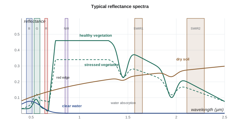
The reflectance of a green leaf is controlled by three things: pigments in the visible, the internal structure of the leaf in the near infrared, and water in the shortwave infrared. In the visible, chlorophyll a and b absorb strongly in the blue near 0.45 µm and in the red near 0.67 µm, and carotenoids absorb in the blue. Green light is absorbed less, giving a small reflectance peak near 0.55 µm, typically 0.08 to 0.15, which is why leaves look green. The red reflectance of a dense healthy canopy is very low, often 0.02 to 0.05.
Beyond about 0.7 µm, pigments stop absorbing, and the reflectance rises steeply in a narrow interval called the red edge. In the near infrared a leaf reflects 40 to 60 % and transmits most of the rest, because light is scattered many times at the boundaries between hydrated cell walls and the air spaces of the spongy mesophyll. A canopy of several leaf layers reflects even more, since light transmitted by one leaf is partly reflected by the leaves below. Near infrared reflectance therefore rises with leaf area and biomass, which is the physical basis of vegetation indices. The position of the red edge shifts slightly toward longer wavelengths as chlorophyll content increases and toward shorter wavelengths under stress, which is why some sensors carry narrow bands between 0.70 and 0.78 µm.
In the shortwave infrared, liquid water in the leaf absorbs strongly, with absorption bands near 1.45 and 1.95 µm, and reflectance at 1.6 and 2.2 µm falls as leaf water content rises. A crop that is short of water first shows a rise in SWIR reflectance, and only later, as cells collapse and chlorophyll breaks down, a rise in red and a fall in near infrared reflectance. Shortwave infrared bands are therefore sensitive to the early stages of water stress that matter for irrigation scheduling.
A canopy is more than a stack of leaves. Its reflectance depends on leaf area index, the one-sided leaf area per unit ground area; on leaf angle, with erect leaves such as wheat reflecting differently from flat leaves such as sugar beet or alfalfa; on the soil visible between the rows, which dominates early in the season; on flowers, seed heads and senescent leaves; and on the sun and view angles, which control how much shadow is seen. Canola in full bloom, for example, is bright yellow and has a much higher green and red reflectance than canola before flowering, so its spectrum changes completely for three weeks in July. Alfalfa is cut several times a year, so a field can go from dense canopy to stubble and back again within a month.
Soil, water, snow and built surfaces
Bare soil generally has a smooth reflectance curve that rises gradually with wavelength, without the sharp red edge of vegetation. Its overall level depends mostly on moisture, organic matter, texture and surface roughness. Moist soil is darker at all wavelengths than the same soil dry, by up to half, and has deeper water absorption features at 1.45 and 1.95 µm. Organic matter darkens soil in the visible; the dark brown and black chernozems of the prairies are darker than the light brown soils of the drier south. Iron oxides produce a reddish color and absorption features near 0.5 and 0.9 µm, and clay minerals have absorption features near 2.2 µm. A freshly cultivated field is rougher and darker than a crusted one, because of its shadows.
Clear water has a low reflectance of a few percent in the blue and green, falling to almost nothing in the near infrared and beyond, where water absorbs strongly. This makes the near infrared and shortwave infrared the best bands for mapping water boundaries: even a shallow flooded field stands out sharply as a dark area. Suspended sediment raises reflectance in the green, red and even near infrared, so the canal after a storm, carrying silt from the coulees, looks brighter and browner than the clear water at the headworks. Chlorophyll in algae raises green reflectance and lowers blue and red, and high concentrations produce a near infrared bump similar to vegetation, which allows algal blooms in reservoirs to be monitored. Surface glint from waves can make water appear bright in any band.
Fresh snow is very bright in the visible, often above 0.9, and much darker in the shortwave infrared because ice absorbs there; clouds are bright in both. The contrast between visible and SWIR reflectance is therefore used to tell snow from cloud in winter and spring images. Concrete, asphalt, gravel and roofs have mostly flat curves at levels that depend on their age and color; new asphalt is dark and becomes lighter with age, and metal roofs can be very bright with strong directional effects. Burned areas show low near infrared and high shortwave infrared reflectance, a combination used in Lesson 8.
Measuring spectra in the field and the laboratory
A field spectroradiometer measures radiance in hundreds of narrow channels. Reflectance is obtained by measuring a reference panel of known, nearly Lambertian reflectance immediately before and after the target, so that the ratio cancels the illumination: \(\rho_{target} = (L_{target}/L_{panel}) \, \rho_{panel}\). The panel must be clean, level and fully lit, and the sky stable, because a cloud passing between the two readings changes the illumination and corrupts the ratio. Measurements are usually made within two hours of solar noon to keep the sun high and shadows short, and several readings over each target are averaged. The instrument's field of view and height determine the footprint, which must be large enough to sample the canopy and soil in their true proportions; a reading of one alfalfa plant is not a reading of an alfalfa field.
Spectral libraries collect measured spectra of minerals, soils, vegetation and man-made materials, and are used to design classifications and to unmix hyperspectral pixels. Library spectra are useful references but rarely match local conditions exactly, so local field spectra like Grant's are preferred for calibrating a project. Field spectra also serve as ground truth for checking atmospheric correction: if the satellite surface reflectance of a large uniform field agrees with the field measurement on the same day, the correction is working.
From spectra to bands
A multispectral sensor does not record a continuous spectrum but integrates the incoming radiance over each band, weighted by the band's spectral response function. The reflectance in a band is therefore an average over the band, and two sensors with slightly different band positions and widths record slightly different reflectances for the same surface. When Leah compared the field spectra with images, she convolved each field spectrum with the response functions of each sensor's bands to simulate what the sensor would see. The differences between sensors are small for broad smooth features and larger where a band falls on a steep part of a curve, such as the red edge.
import math
# Surface reflectance (0-1) at six band centres, typical mid-July values for the canal service area
bands = ["blue 0.49", "green 0.56", "red 0.665", "NIR 0.842", "SWIR1 1.61", "SWIR2 2.19"]
lib = {
    "irrigated alfalfa": [0.030, 0.075, 0.035, 0.480, 0.200, 0.090],
    "irrigated wheat":   [0.035, 0.070, 0.045, 0.390, 0.230, 0.120],
    "canola in bloom":   [0.050, 0.150, 0.060, 0.420, 0.240, 0.120],
    "dryland stubble":   [0.090, 0.130, 0.170, 0.250, 0.340, 0.270],
    "bare clay soil":    [0.100, 0.140, 0.180, 0.230, 0.300, 0.250],
    "canal water":       [0.060, 0.070, 0.040, 0.020, 0.008, 0.005],
}
def nd(a, b): return (a - b) / (a + b)
print(f"{'cover':18s}  NDVI    NDWI   NDMI")
for name, r in lib.items():
    print(f"{name:18s} {nd(r[3], r[2]):6.3f} {nd(r[1], r[3]):6.3f} {nd(r[3], r[4]):6.3f}")

def sam(a, b):
    dot = sum(x * y for x, y in zip(a, b))
    na = math.sqrt(sum(x * x for x in a)); nb = math.sqrt(sum(y * y for y in b))
    return math.degrees(math.acos(min(1.0, dot / (na * nb))))

print()
print("Spectral angle (deg) between covers")
names = list(lib)
for i in range(len(names)):
    for j in range(i + 1, len(names)):
        print(f"  {names[i]:18s} vs {names[j]:18s} {sam(lib[names[i]], lib[names[j]]):5.1f}")

# Which single band separates alfalfa from wheat best, relative to a 0.015 field-to-field spread?
print()
a, w = lib["irrigated alfalfa"], lib["irrigated wheat"]
for bnd, x, y in zip(bands, a, w):
print(f"{bnd:11s} difference {x - y:+.3f} separability {abs(x - y) / 0.015:4.1f} spreads")cover NDVI NDWI NDMI irrigated alfalfa 0.864 -0.730 0.412 irrigated wheat 0.793 -0.696 0.258 canola in bloom 0.750 -0.474 0.273 dryland stubble 0.190 -0.316 -0.153 bare clay soil 0.122 -0.243 -0.132 canal water -0.333 0.556 0.429 Spectral angle (deg) between covers irrigated alfalfa vs irrigated wheat 9.3 irrigated alfalfa vs canola in bloom 12.2 irrigated alfalfa vs dryland stubble 38.7 irrigated alfalfa vs bare clay soil 39.8 irrigated alfalfa vs canal water 68.6 irrigated wheat vs canola in bloom 8.4 irrigated wheat vs dryland stubble 30.0 irrigated wheat vs bare clay soil 31.6 irrigated wheat vs canal water 67.2 canola in bloom vs dryland stubble 29.4 canola in bloom vs bare clay soil 30.1 canola in bloom vs canal water 60.3 dryland stubble vs bare clay soil 4.1 dryland stubble vs canal water 57.7 bare clay soil vs canal water 54.0 blue 0.49 difference -0.005 separability 0.3 spreads green 0.56 difference +0.005 separability 0.3 spreads red 0.665 difference -0.010 separability 0.7 spreads NIR 0.842 difference +0.090 separability 6.0 spreads SWIR1 1.61 difference -0.030 separability 2.0 spreads SWIR2 2.19 difference -0.030 separability 2.0 spreads
The output shows which bands carry the information. Alfalfa and wheat differ hardly at all in the blue, green and red bands, by less than the field-to-field spread of about 0.015, but by six spreads in the near infrared and by two in each shortwave band. The spectral angle, which compares the shape of two curves regardless of brightness, separates the vegetated covers from soil and water by 30 to 70 degrees but alfalfa, wheat and canola by only 8 to 12 degrees, and dryland stubble from bare soil by only 4 degrees. A single date is therefore enough to separate green from not green, but the crops themselves need several dates, which the classification lesson will use.
Spectral indices
A spectral index combines two or more bands into a single number that emphasizes one property and suppresses others, such as illumination differences and some atmospheric effects. The most widely used is the normalized difference vegetation index:
NDVI ranges from −1 to +1. Water usually has negative values, bare soil and rock values near 0.1 to 0.2, sparse vegetation 0.2 to 0.5 and dense green canopies 0.6 to 0.9. Because it is a ratio, NDVI partly cancels differences in illumination caused by slope and sun angle. It has known weaknesses: it saturates over dense canopies, rising little once leaf area index exceeds about 3, and it is affected by the color and brightness of the soil beneath sparse canopies. Many alternatives have been proposed to address these weaknesses.
| Index | Formula | Sensitive to | Notes |
|---|---|---|---|
| NDVI | (NIR − red)/(NIR + red) | Green vegetation amount | Saturates over dense canopy; affected by soil |
| SAVI | 1.5 (NIR − red)/(NIR + red + 0.5) | Vegetation over bright soil | Soil-adjusted with L = 0.5 |
| EVI | 2.5 (NIR − red)/(NIR + 6 red − 7.5 blue + 1) | Dense vegetation | Less saturation; corrects some aerosol effect |
| NDWI (McFeeters) | (green − NIR)/(green + NIR) | Open water | Positive over water |
| NDMI | (NIR − SWIR1)/(NIR + SWIR1) | Canopy water content | Also called NDWI (Gao); useful for irrigation status |
| NBR | (NIR − SWIR2)/(NIR + SWIR2) | Burned areas | Used for burn severity in Lesson 8 |
| NDRE | (NIR − red edge)/(NIR + red edge) | Chlorophyll in dense canopy | Needs a red edge band |
Worked problem
NDVI and NDMI of an irrigated and a dry field
In a July image, an irrigated wheat field has reflectances red 0.045, NIR 0.390 and SWIR1 0.230. A neighboring dryland wheat field has red 0.070, NIR 0.310 and SWIR1 0.300. Compute NDVI and NDMI for both and comment.
Show solution
- \[\text{NDVI}_{irr} = \frac{0.390 - 0.045}{0.390 + 0.045} = \frac{0.345}{0.435} = 0.793\]
- \[\text{NDVI}_{dry} = \frac{0.310 - 0.070}{0.310 + 0.070} = \frac{0.240}{0.380} = 0.632\]
- \[\text{NDMI}_{irr} = \frac{0.390 - 0.230}{0.390 + 0.230} = 0.258, \quad \text{NDMI}_{dry} = \frac{0.310 - 0.300}{0.610} = 0.016\]
Answer: Both fields are green, but the dry field's NDMI is near zero while the irrigated field's is clearly positive. The relative difference in NDMI is much larger than in NDVI, which is why moisture-sensitive indices are useful for mapping irrigation.
How signatures change over time
A crop's spectrum follows a seasonal path called its phenology. A spring wheat field is bare soil in May, shows rising NDVI from emergence in late May to a peak at heading in early July, and then falls as the crop ripens and turns golden before harvest in August. Canola emerges later, peaks in July with a distinctive yellow flowering stage, and is swathed in late August. Alfalfa is green from early spring, falls sharply at each cut and recovers within two or three weeks. Winter wheat greens up early, ripens by late July and is often harvested before spring crops peak. Irrigated fields stay green later into the season than dryland fields of the same crop.
These differences in timing are often more diagnostic than any single-date spectrum. An NDVI profile through the season, built from many cloud-free images, is a signature in time as well as wavelength. The district's crop map would be built from such profiles, and the dates of the field visits would be chosen to coincide with the stages at which the crops differ most: canola flowering, the wheat and barley ripening, and the regrowth of alfalfa after a cut.
Common mistakes
MistakeAssuming that one class has one spectrum.
InsteadEach class has a family of spectra that varies with growth stage, moisture, management and viewing geometry; sample that variation.
MistakeMeasuring field spectra with a dirty or shaded reference panel.
InsteadKeep the panel clean, level and in full sun, and repeat panel readings whenever the light changes.
MistakeUsing the term NDWI without a formula.
InsteadState the bands used; two different indices share the name.
MistakeReading high NDVI as high yield or adequate water.
InsteadNDVI measures green cover; use SWIR or thermal information, and field data, for water status.
MistakeComparing reflectances from sensors with different band positions without adjustment.
InsteadAccount for spectral response differences, especially near the red edge.
Summary and key terms
- A spectral signature is a reflectance curve against wavelength; each class has a family of curves rather than one fixed curve.
- Green vegetation has low red and blue reflectance from chlorophyll absorption, a steep red edge and high NIR reflectance from leaf structure.
- Leaf water absorbs in the SWIR, so SWIR reflectance rises as plants dry.
- Soil reflectance rises smoothly with wavelength and falls with moisture and organic matter; water is dark in the NIR and SWIR.
- Field spectra are measured relative to a calibrated reference panel.
- Spectral indices such as NDVI, NDMI and NBR condense band information into a single number.
- Seasonal change, or phenology, is often more diagnostic than a single-date spectrum.
- Spectral signature
- The pattern of reflectance of a surface as a function of wavelength.
- Red edge
- The steep rise in vegetation reflectance between about 0.68 and 0.75 µm.
- Leaf area index
- The one-sided green leaf area per unit ground area.
- Spectral response function
- The relative sensitivity of a sensor band at each wavelength.
- NDVI
- The normalized difference vegetation index, (NIR − red)/(NIR + red).
- Phenology
- The seasonal timing of plant growth stages and the spectral changes that accompany them.
- Spectral angle
- The angle between two spectra treated as vectors, which measures difference in shape regardless of brightness.
Practice problems
Work each problem on paper first, then reveal the answer to check.
A canopy has red reflectance 0.04 and NIR 0.44. What is its NDVI?
Show answer
(0.44 − 0.04)/(0.44 + 0.04) = 0.833.
Compute SAVI for the same canopy with L = 0.5.
Show answer
1.5 × 0.40 / (0.48 + 0.5) = 0.612.
A target reads 0.36 of the panel radiance, and the panel reflectance is 0.98. What is the target reflectance?
Show answer
0.36 × 0.98 = 0.353.
Why is the NIR band better than the green band for mapping a flooded field?
Show answer
Water is nearly black in the NIR, while vegetation and soil are bright, so the contrast is far greater.
Which change appears first in an alfalfa field running short of water: higher SWIR reflectance or lower NIR reflectance?
Show answer
Higher SWIR reflectance, as leaf water content drops before the canopy structure and chlorophyll change.
Lesson quiz · 5 questions
Score 60% or more to complete this lesson.
Create a free account to save your progress, take quizzes and earn a certificate.