
GEOM-320 · Lesson 4 of 12 · 21 min
Resolution
When Leah presented the data sources, a board member asked the obvious question: why not simply buy the sharpest images available? The answer took the rest of the meeting. The service area has about 1,100 fields, many of them quarter sections of 64 ha under center pivots, but also narrow strips along the coulees, small vegetable plots and the canal itself, which is 24 m wide at the water surface. The program needed to see crops change within days, distinguish irrigated from dry fields by subtle differences in moisture and temperature, and keep the cost of data and processing within the budget. Every one of these needs pulls on a different kind of resolution. This lesson explains the four resolutions of a remote sensing system, spatial, spectral, radiometric and temporal, how they are defined and measured, and why they cannot all be maximized at once.
Spatial resolution
Spatial resolution describes the size of the smallest feature that can be detected or measured. It is commonly quoted as the ground sample distance (GSD), the spacing between pixel centers on the ground, but GSD is only part of the story. The instantaneous field of view (IFOV) of a detector is the angle it subtends, and at nadir its ground footprint is approximately \(H \cdot \text{IFOV}\), where \(H\) is the altitude. For Landsat's Operational Land Imager at 705 km, an IFOV of about 42.5 microradians gives a 30 m footprint. Pixels at the edge of a wide swath look obliquely and cover more ground; for a sensor with a ±55° scan, such as the weather satellite imagers, edge pixels are several times larger than nadir pixels unless the design compensates.
A sharper description is the point spread function (PSF), the image of an infinitely small bright point. Optics, detector size, platform motion, electronics and the atmosphere all blur the image, so each pixel collects some light from its neighbors. The modulation transfer function (MTF), the Fourier transform of the PSF, gives the contrast with which patterns of different spatial frequency are reproduced; a well-designed sensor has an MTF of 0.2 to 0.3 at its Nyquist frequency, the pattern with a period of two pixels. Two sensors with the same GSD can therefore differ in effective sharpness, and resampling an image to a smaller pixel size does not create detail that the sensor did not record.
A related idea is the difference between detection and identification. A feature smaller than a pixel can be detected if it contrasts strongly with its surroundings: a hot fire covering a few square meters raises the temperature of a 1 km thermal pixel enough to trigger a fire detection, and a narrow canal shows clearly in a 30 m near infrared image because water is so dark. Identifying what a feature is, or measuring its size, needs several pixels across it. A common rule of thumb is that measuring a feature's area to within 10 % needs it to span at least several tens of pixels.
Mixed pixels
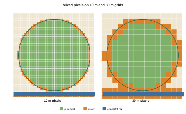
Most pixels in an agricultural landscape contain more than one cover: field edges, farmyards, roads, shelterbelts, ditches and canal banks all create mixed pixels whose reflectance is a weighted combination of the covers inside them. At 30 m, a pivot field has a ring of mixed pixels around its edge and a corner of dryland or grass in each square quarter section; at 250 m, few pixels are pure. Mixed pixels blur boundaries, cause misclassification at edges and bias area estimates if they are assigned whole to one class. The linear mixture model of Lesson 10 treats a mixed pixel's spectrum as the area-weighted sum of pure endmember spectra and estimates the fractions.
Spectral resolution
Spectral resolution describes the number, width and placement of the bands. A panchromatic band covers much of the visible and near infrared in one broad band; a multispectral sensor has a handful to a dozen or so bands, each typically 20 to 100 nm wide; a hyperspectral sensor has 100 to 300 or more contiguous bands, each about 5 to 10 nm wide. The width of a band is usually given as its full width at half maximum, the interval over which the spectral response exceeds half its peak. Narrow, well-placed bands can capture features such as the red edge, the chlorophyll absorption or the clay absorption at 2.2 µm that broad bands average away. Placement matters as much as width: Landsat's SWIR bands were chosen to measure leaf and soil moisture, and its cirrus band to detect thin cloud.
Narrow bands collect less light, so for a given detector and integration time they have a lower signal-to-noise ratio, or they need larger pixels to collect enough. This is one reason hyperspectral satellites commonly have 30 m pixels while multispectral sensors reach 10 m and panchromatic bands reach sub-meter resolution. Pansharpening, covered in Lesson 6, exploits the trade by combining a sharp panchromatic band with coarser color bands.
Radiometric resolution
Radiometric resolution describes how finely a sensor distinguishes differences in brightness. It is often quoted as the number of bits per pixel: an 8-bit sensor records 256 levels, a 12-bit sensor 4,096 and a 14-bit sensor 16,384. Landsat 8 records 12 bits and Landsat 9 14 bits, and Sentinel-2 records 12 bits. Bits alone do not guarantee sensitivity; what matters is the signal-to-noise ratio at typical radiance levels and the noise-equivalent change in reflectance or temperature. A sensor with many bits but high noise records its noise very precisely. For thermal sensors the corresponding measure is the noise-equivalent differential temperature (NEΔT), about 0.1 K or better for modern thermal satellite instruments.
Radiometric resolution matters most over dark targets such as water, where the signal occupies only the lowest levels, and for detecting small changes, such as the slight drop in NIR reflectance that precedes visible stress. The older 8-bit sensors often saturated over bright snow and cloud and lacked detail in water; 12-bit and 14-bit data make it possible to map water quality and shadows with confidence. Radiometric accuracy, the agreement of calibrated values with the truth, is a separate property that depends on calibration rather than on the number of levels.
Temporal resolution
Temporal resolution is the interval between successive observations of the same place. For a single satellite it is set by the repeat cycle, but in practice it is reduced by combining satellites and increased by cloud. A program that needs a clear image of every field within a two-week window in June needs several opportunities in that window, because the probability that any one overpass is clear is well below one. Satellites with pointable sensors can revisit more often than their repeat cycle, at the cost of oblique views. For radar, cloud does not matter, but repeat geometry does: interferometry requires images from the same orbit track, so the useful interval is the exact repeat cycle.
Temporal resolution must match the speed of the process being watched. Canal levels and flooded fields change in hours; crops change in days; the coulee banks move a few millimeters a month; land use changes over years. Matching the observation interval to the process avoids both missing events and paying for redundant data.
import math
# Spatial: ground sample distance from the instantaneous field of view
for name, h_km, ifov_urad in (("Landsat OLI", 705, 42.5), ("Sentinel-2 MSI 10 m bands", 786, 12.7), ("MODIS 250 m bands", 705, 354.0)):
    print(f"{name:26s} IFOV {ifov_urad:6.1f} urad at {h_km} km -> GSD {h_km * 1000 * ifov_urad * 1e-6:6.1f} m")

# Mixed pixels: a square field 400 m on a side on a grid of pixel size p (field edges not aligned)
print()
print("pixel  pixels touching field  pure field pixels  share of field area in pure pixels")
side = 400.0
for p in (3.0, 10.0, 30.0, 250.0):
    n_touch = math.ceil(side / p + 1) ** 2
    n_pure = max(0, math.floor(side / p - 1)) ** 2
    print(f"{p:5.0f} m  {n_touch:10d}            {n_pure:8d}           {n_pure * p * p / side**2 * 100:6.1f} %")

# Radiometric: quantization levels and the smallest reflectance step
print()
for bits in (8, 12, 14, 16):
    lv = 2 ** bits
    print(f"{bits:2d} bits: {lv:6d} levels, step {1.0 / (lv - 1):.6f} over a 0-1 reflectance range")

# Temporal: chance of at least one clear view in a 10-day window
print()
p_clear = 0.40      # probability that a single overpass is clear over the field in June
for name, revisit in (("Landsat 8/9 (8 d)", 8), ("Sentinel-2 pair (about 3 d at this latitude)", 3), ("daily small-satellite fleet", 1)):
    n = 10 // revisit
    print(f"{name:44s} {n:2d} looks, P(at least one clear) = {1 - (1 - p_clear) ** n:5.3f}")

# Data volume for one 100 km x 100 km scene
print()
for name, p, nb, bits in (("10 m, 4 bands, 12 bit", 10, 4, 12), ("30 m, 11 bands, 12 bit", 30, 11, 12), ("30 m hyperspectral, 220 bands, 14 bit", 30, 220, 14)):
    px = (100000 / p) ** 2
print(f"{name:40s} {px * nb * bits / 8 / 1e6:8.0f} MB")Landsat OLI IFOV 42.5 urad at 705 km -> GSD 30.0 m
Sentinel-2 MSI 10 m bands IFOV 12.7 urad at 786 km -> GSD 10.0 m
MODIS 250 m bands IFOV 354.0 urad at 705 km -> GSD 249.6 m
pixel pixels touching field pure field pixels share of field area in pure pixels
3 m 18225 17424 98.0 %
10 m 1681 1521 95.1 %
30 m 225 144 81.0 %
250 m 9 0 0.0 %
8 bits: 256 levels, step 0.003922 over a 0-1 reflectance range
12 bits: 4096 levels, step 0.000244 over a 0-1 reflectance range
14 bits: 16384 levels, step 0.000061 over a 0-1 reflectance range
16 bits: 65536 levels, step 0.000015 over a 0-1 reflectance range
Landsat 8/9 (8 d) 1 looks, P(at least one clear) = 0.400
Sentinel-2 pair (about 3 d at this latitude) 3 looks, P(at least one clear) = 0.784
daily small-satellite fleet 10 looks, P(at least one clear) = 0.994
10 m, 4 bands, 12 bit 600 MB
30 m, 11 bands, 12 bit 183 MB
30 m hyperspectral, 220 bands, 14 bit 4278 MBThe code quantifies the trade-offs. A 400 m field is 98 % pure at 3 m and 95 % at 10 m, but only 81 % at 30 m and not at all at 250 m, where every pixel is mixed. With a 40 % chance of a clear sky on any one pass, a single Landsat look in a 10-day window succeeds only 40 % of the time, three Sentinel-2 looks 78 % of the time and a daily constellation almost always. Data volume grows with the square of the inverse pixel size and in proportion to the number of bands and bits, so a 30 m hyperspectral scene with 220 bands is over 20 times the size of a 30 m multispectral scene.
Worked problem
Footprint and pure pixels
A thermal sensor at 705 km has an IFOV of 142 µrad. What is its ground footprint at nadir? How many fully pure footprints fit across a 400 m square field if the grid is not aligned with the field?
Show solution
- \[\text{footprint} = H \cdot \text{IFOV} = 705{,}000 \times 142 \times 10^{-6} = 100.1 \text{ m}\]
- \[\text{pure pixels across} = \lfloor 400 / 100 - 1 \rfloor = 3\]
- \[\text{pure pixels in the field} = 3^2 = 9, \quad \text{pure share} = \frac{9 \times 100^2}{400^2} = 56 \%\]
Answer: Only about half of the field is covered by pure thermal pixels at 100 m, so water use estimates for single fields must use only interior pixels or sharpen the thermal data with finer optical bands.
Trade-offs and choices
The four resolutions compete. Finer spatial resolution means smaller pixels, which collect less energy, so narrower bands or more bits become harder to achieve. A wide swath, which gives frequent coverage, means more detectors or larger pixels and higher data rates. Data downlink capacity and onboard storage limit how much of everything can be recorded. The table summarizes how the needs of the district's products mapped to resolutions.
| Product | Spatial | Spectral | Temporal | Radiometric |
|---|---|---|---|---|
| Crop type map | 10 to 30 m | Visible, red edge, NIR, SWIR | Several dates over the season | 12 bits adequate |
| Irrigation status | 10 to 30 m | NIR and SWIR | Every 1 to 2 weeks | Low noise in SWIR |
| Crop water use | 30 to 100 m thermal | Thermal plus reflective | Weekly in summer | NEΔT about 0.1 K |
| Bank movement | Meters (radar) | One radar band | Monthly or better, same geometry | Phase stability |
| Flood extent | 5 to 30 m | Radar or NIR | Hours to a day during an event | Moderate |
| Structure condition | Sub-meter | True color | Annual or on demand | Moderate |
Leah's conclusion for the board was that no single sensor could serve every product, and that the sharpest images were the right choice only for a few small tasks. Sentinel-2 at 10 m offered the best balance for field-level crop and irrigation products, Landsat thermal data at 100 m were adequate for water use if interior pixels were used, and radar was needed for the banks and floods. Field size also guided the choice: most fields in the service area were large enough for 10 m and even 30 m pixels, but the small vegetable plots near the town would need commercial imagery or would be reported as a mixed class.
Common mistakes
MistakeEquating GSD with resolving power.
InsteadEffective resolution also depends on the point spread function; resampling to smaller pixels does not add detail.
MistakeAssuming that more bits mean better data.
InsteadSignal-to-noise ratio determines sensitivity; noisy high-bit data are not better than clean lower-bit data.
MistakePlanning on the repeat cycle alone.
InsteadAccount for cloud with the probability of clear observations within the needed window.
MistakeEstimating field areas by counting all pixels touched by a field.
InsteadMixed edge pixels inflate the area; use pure pixels, fractions or vector boundaries.
MistakeChoosing the finest resolution available for every task.
InsteadMatch each resolution to the size and speed of the process; finer data increase cost and processing.
Summary and key terms
- Spatial resolution is described by GSD, IFOV, the point spread function and the MTF.
- Features smaller than a pixel can be detected if contrast is high, but identification and measurement need several pixels.
- Mixed pixels are common at field edges and grow in share as pixel size increases.
- Spectral resolution is the number, width and placement of bands; hyperspectral sensors trade spatial resolution for narrow bands.
- Radiometric resolution is set by quantization and, more importantly, signal-to-noise ratio or NEΔT.
- Temporal resolution depends on repeat cycles, constellations, pointing and cloud.
- The four resolutions trade against each other and must be matched to the needs of each product.
- Ground sample distance
- The distance on the ground between the centers of adjacent pixels.
- Instantaneous field of view
- The angular field of view of a single detector element.
- Point spread function
- The image of a point source, describing how a sensor blurs the scene.
- Mixed pixel
- A pixel whose area contains more than one surface cover.
- Full width at half maximum
- The width of a spectral band between the points where its response is half its peak.
- NEΔT
- Noise-equivalent differential temperature, the temperature difference that produces a signal equal to the noise.
Practice problems
Work each problem on paper first, then reveal the answer to check.
What is the nadir footprint of a 12.7 µrad detector at 786 km?
Show answer
786,000 × 12.7 × 10⁻⁶ = 10.0 m.
How many pixels of 10 m cover a 64 ha field?
Show answer
640,000 m² / 100 m² = 6,400.
A 14-bit sensor records reflectance from 0 to 1. What is the smallest step?
Show answer
1/16,383 = 0.000061.
The chance of a clear sky on each pass is 0.5. How many independent passes give a 95 % chance of at least one clear image?
Show answer
1 − 0.5ⁿ ≥ 0.95, so n = 5.
Why does a 24 m wide canal appear in a 30 m NIR image although it is narrower than a pixel?
Show answer
Water is so dark in the NIR that even partial cover lowers the pixel reflectance clearly; it is detected but not measured.
Lesson quiz · 5 questions
Score 60% or more to complete this lesson.
Create a free account to save your progress, take quizzes and earn a certificate.