Image enhancement

The first image Theo put on the screen for the board looked gray and flat: a corrected 12-bit Sentinel-2 scene displayed without any stretch occupied only the lowest tenth of the display range. Ten minutes later the same data, stretched and shown as a false-color composite, made the irrigated fields glow red against the brown stubble and the dark blue canal, and the board members began pointing out their own fields. Enhancement changes how data look, not what they are, but it decides what an analyst or a client can see. This lesson covers color composites, contrast enhancement, spatial filtering, band arithmetic, principal components and pansharpening, and the rules for using them honestly.

Displaying multispectral data

A computer display has three color channels, red, green and blue, each typically with 256 levels. A color composite assigns one band to each channel. A true-color or natural-color composite assigns the red band to red, green to green and blue to blue, giving an image that looks roughly as the eye would see it, usually hazy and low in contrast because of atmospheric scattering in the blue. The standard false-color composite assigns near infrared to red, red to green and green to blue. Healthy vegetation, bright in the NIR, appears red; bare soil appears blue-gray or brown; water appears dark blue or black; and urban areas appear cyan. Other combinations serve particular purposes: SWIR, NIR and red shows moisture differences and burn scars clearly; SWIR2, SWIR1 and red is used for geology and to see through thin smoke, because SWIR wavelengths scatter far less than visible ones.

Color composites exploit the eye's sensitivity to color differences, which is greater than its sensitivity to differences in gray level. But the colors are arbitrary, and a board member who has not been told that red means vegetation may conclude that the fields are on fire. Every product delivered to a client should therefore state the band combination in its legend.

Contrast enhancement

The values in a band rarely fill the full display range. A corrected 12-bit band of an agricultural scene may occupy 400 to 3,000 of 4,096 possible values in the NIR and only 200 to 1,200 in the red. Contrast enhancement maps the data values to display values so that the range of interest fills the display. The image histogram, the count of pixels at each value, guides the choice.

A linear stretch maps a chosen minimum and maximum to 0 and 255 and scales linearly between them; values outside are clipped. Choosing the minimum and maximum at the 2nd and 98th percentiles rather than at the extreme values prevents a few very bright or dark pixels, such as cloud or deep shadow, from compressing the rest. A piecewise linear stretch uses different slopes over different parts of the range, for example to expand the dark values of water while keeping the land readable. Histogram equalization maps each value to its cumulative frequency, so that each display level is used by roughly the same number of pixels; it brings out detail in the most common values and compresses rare ones, which can exaggerate small differences in large uniform areas. Gamma and logarithmic stretches compress bright values and expand dark ones.

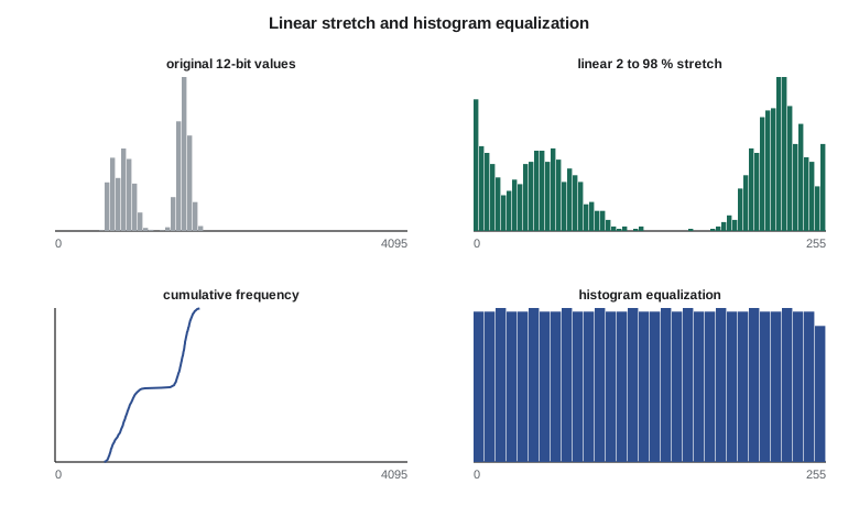
Contrast enhancement is for display only. Stretched values have lost their physical meaning: a pixel of 200 in one stretched image and 200 in another need not have the same reflectance. All measurements, indices and classifications must use the calibrated values, not the stretched ones.

Spatial filtering

Spatial filters change each pixel according to its neighbors, usually by convolution with a small kernel. A low-pass filter, such as the 3 × 3 mean or a Gaussian, smooths the image, reducing noise and fine detail. The median filter, which replaces each pixel by the median of its neighborhood, removes isolated spikes and speckle while preserving edges better than the mean; it is widely used on radar images and on classified maps to remove isolated misclassified pixels. A high-pass filter emphasizes local differences: subtracting a smoothed version from the original leaves the fine detail, and adding some of that detail back sharpens the image. Edge-detection filters, such as the Sobel operators, estimate the gradient in the row and column directions; the magnitude of the gradient is large along boundaries such as field edges, roads and the canal banks.

Filtering is also done in the frequency domain with the Fourier transform. Periodic noise, such as striping from detector differences, appears as isolated spikes in the Fourier spectrum and can be removed by masking those frequencies and transforming back. Texture measures, such as the local variance or measures derived from the gray-level co-occurrence matrix, describe how values vary within a window and help separate covers with similar average reflectance but different structure, such as a shelterbelt and an irrigated field.

# A small 8 x 8 window of a 12-bit red band over the canal, a road and fields (top-of-atmosphere DN)
img = [
    [812, 820, 835, 840, 1490, 1502, 1515, 1498],
    [808, 815, 830, 845, 1485, 1510, 1520, 1505],
    [790, 800, 812, 1180, 1470, 1495, 1508, 1512],
    [640, 655, 690, 1150, 1460, 1488, 1501, 1499],
    [610, 620, 645, 1120, 1452, 1477, 1494, 1490],
    [905, 910, 930, 1210, 1600, 1655, 1670, 1660],
    [920, 925, 940, 1230, 1640, 1680, 1690, 1685],
    [930, 935, 950, 1240, 1650, 1700, 1710, 1702],
]
flat = sorted(v for r in img for v in r)
def pct(p):
    i = (len(flat) - 1) * p / 100.0
    lo = int(i); hi = min(lo + 1, len(flat) - 1)
    return flat[lo] + (flat[hi] - flat[lo]) * (i - lo)
lo, hi = pct(2), pct(98)
print(f"2nd and 98th percentiles: {lo:.1f} and {hi:.1f}")
def stretch(v): return max(0, min(255, round((v - lo) / (hi - lo) * 255)))
print("\nLinear 2-98 % stretch to 0-255:")
for r in img: print(" ".join(f"{stretch(v):4d}" for v in r))

# Histogram equalization: map each value to its cumulative frequency
n = len(flat)
cdf = {}
for i, v in enumerate(flat): cdf[v] = (i + 1) / n
print("\nHistogram equalization to 0-255:")
for r in img: print(" ".join(f"{round(cdf[v] * 255):4d}" for v in r))

# 3 x 3 filters on the interior pixels
def conv(k):
    out = []
    for i in range(1, 7):
        out.append([sum(k[a][b] * img[i - 1 + a][j - 1 + b] for a in range(3) for b in range(3)) for j in range(1, 7)])
    return out
mean = conv([[1 / 9] * 3] * 3)
gx = conv([[-1, 0, 1], [-2, 0, 2], [-1, 0, 1]])
gy = conv([[-1, -2, -1], [0, 0, 0], [1, 2, 1]])
print("\n3 x 3 mean (interior):")
for r in mean: print(" ".join(f"{v:6.0f}" for v in r))
print("\nSobel gradient magnitude (interior):")
for a, b in zip(gx, gy): print(" ".join(f"{(x * x + y * y) ** 0.5:6.0f}" for x, y in zip(a, b)))

2nd and 98th percentiles: 625.2 and 1701.5

Linear 2-98 % stretch to 0-255:
  44   46   50   51  205  208  211  207
  43   45   49   52  204  210  212  208
  39   41   44  131  200  206  209  210
   4    7   15  124  198  204  208  207
   0    0    5  117  196  202  206  205
  66   67   72  139  231  244  248  245
  70   71   75  143  240  250  252  251
  72   73   77  146  243  255  255  255

Histogram equalization to 0-255:
  44   52   60   64  159  183  203  171
  36   48   56   68  147  195  207  187
  28   32   44  116  139  167  191  199
  12   20   24  112  135  151  179  175
   4    8   16  108  131  143  163  159
  72   76   92  120  211  223  231  227
  80   84  100  124  215  235  243  239
  92   96  104  128  219  247  255  251

3 x 3 mean (interior):
   814    864   1087   1313   1499   1507
   760    864   1102   1343   1493   1504
   696    852   1109   1366   1483   1496
   734    881   1140   1401   1533   1548
   823    948   1196   1452   1595   1611
   927   1030   1266   1512   1666   1684

Sobel gradient magnitude (interior):
   123    535   2699   2326    139      8
   639   1292   2777   1650    176     77
   724   1956   3020   1353    176     86
  1025   1963   3095   1581    672    667
  1220   1727   2933   1832    823    790
   127   1219   2773   1813    292    168

The 8 × 8 window shows three areas: dark canal water at the left, a field on the right and the road between them. The linear stretch maps the canal to near zero and the brightest field values to 255 while keeping their spacing proportional. Equalization spreads the canal and field values more evenly across the range, so differences within the field become more visible, but the large jump across the road shrinks in relative terms. The mean filter blurs the road into the field, and the Sobel magnitude is largest in the column of the road, where the brightness changes most, which is exactly how edges are found automatically.

Band arithmetic and indices

Arithmetic between bands produces new images. Ratios such as NIR/red, or normalized differences such as NDVI, emphasize differences in spectral shape and suppress differences in overall brightness, including those caused by slope illumination: a shaded slope reduces both bands by about the same factor, so their ratio changes little. Because path radiance is additive rather than multiplicative, ratios computed from uncorrected data are biased, especially for dark targets, so ratios should be computed from surface reflectance. Differences between dates, the subject of Lesson 8, are also band arithmetic.

Principal components and transformations

Neighboring bands are often strongly correlated: the blue, green and red bands of a crop scene rise and fall together. Principal component analysis (PCA) rotates the band space so that the first component, a weighted sum of all bands, carries the largest possible share of the variance, the second carries the largest share of what remains and is uncorrelated with the first, and so on. For a typical six-band scene the first component, close to overall brightness, carries 80 to 90 % of the variance, and the last components carry mostly noise. PCA is used to compress data, to reduce noise by discarding the last components, and in change detection, where components computed from a two-date stack can isolate change. Its components depend on the scene statistics, so they are not comparable between scenes.

Fixed transformations avoid that dependence. The tasseled cap transformation uses published coefficients for each sensor to produce brightness, greenness and wetness components with consistent meanings in agricultural scenes; its wetness component, which contrasts the SWIR bands with the visible and NIR, is sensitive to soil and canopy moisture and has been used to map irrigation. Color space transformations from red-green-blue to intensity, hue and saturation separate brightness from color and underlie some pansharpening methods.

Pansharpening

Many sensors record a panchromatic band at higher spatial resolution than their multispectral bands: Landsat 8 and 9 at 15 m against 30 m, and commercial satellites at 30 to 50 cm against 1.2 to 2 m. Pansharpening combines them to produce a multispectral image with the panchromatic band's spatial detail. Component-substitution methods transform the multispectral bands, replace the intensity or first principal component with the panchromatic band after matching its histogram, and transform back. Multiresolution methods extract the high-frequency detail of the panchromatic band with a filter and inject it into each upsampled multispectral band. The Brovey and intensity substitution methods give sharp images with strong color distortion where the panchromatic band's spectral range differs from the multispectral bands; detail-injection methods preserve color better. A pansharpened image is good for interpretation and digitizing, but the injected detail is not a measurement in each band, so quantitative work should use the original multispectral values.

Using enhancement honestly

Leah set three rules for the program's products. Every display product would state its band combination and stretch. No analysis would use stretched or pansharpened values. And when two dates were shown side by side for the board, both would use the same stretch, computed from the combined histogram of the two images, so that a difference in appearance would reflect a difference in the land rather than in the display settings. Theo added a fourth, practical rule: images shown in the meetings would use color schemes that remained readable to board members with red-green color vision deficiency, which ruled out several popular vegetation index palettes.